Ultrasound-guided prostate percutaneous intervention robot system and calibration by informative particle swarm optimization

Abstract

Applying a robot system in ultrasound-guided percutaneous intervention is an effective approach for prostate cancer diagnosis and treatment. The limited space for robot manipulation restricts structure volume and motion. In this paper, an 8-degree-of-freedom robot system is proposed for ultrasound probe manipulation, needle positioning, and needle insertion. A novel parallel structure is employed in the robot system for space saving, structural rigidity, and collision avoidance. The particle swarm optimization method based on informative value is proposed for kinematic parameter identification to calibrate the parallel structure accurately. The method identifies parameters in the modified kinematic model stepwise according to parameter discernibility. Verification experiments prove that the robot system can realize motions needed in targeting. By applying the calibration method, a reasonable, reliable forward kinematic model is built, and the average errors can be limited to 0.963 and 1.846 mm for insertion point and target point, respectively.

Key words： ultrasound image guidance; prostate percutaneous intervention; parallel robot; kinematics identification; particle swarm optimization; informative value

1 Introduction

Prostate cancer is a widespread disease that threatens men’s health [1]. Transrectal ultrasonography (TRUS)-guided biopsy and brachytherapy are effective approaches for prostate diagnosis and treatment [2]. To accomplish these procedures, feasible and reliable prostate percutaneous intervention is needed. Generally, the physician operates an ultrasound probe and inserts a needle simultaneously with the help of a tablet. The insertion trail is restricted in the ultrasound probe imaging plane to help the physician reduce insertion difficulty, but the restriction reduces insertion flexibility [3]. Moreover, the insertion procedure needs repetitive attempts and greatly depends on the operator’s experience. To reduce experience dependence, manipulation difficulty, and patient trauma, and increase insertion accuracy and manipulation flexibility, image-guided percutaneous intervention robots are developed [4], and an automatic ultrasound-guided prostate intervention is the basis for further medical image fusion application [5,6].

Researchers have proposed different varieties of prostate robot systems. Robot “Apollo” was designed with three motors and three brakes to manipulate the endorectal ultrasound probe [7]. The structure employed transrectal access and could realize remote center motion. A 9-degree-of-freedom (9-DOF) structure for prostate brachytherapy was proposed to manipulate the ultrasound probe and adjust the tablet for needle attitude guidance [3]. The structure worked with a high flexibility, but the overlarge size limited its practical application. In Ref. [8], a 4-DOF hands-free probe manipulator for TRUS-guided prostate biopsy was designed. The needle driver employed transrectal access and was coupled with the probe motion. In addition to the customized manipulators, commercial robots were employed as assistance to manipulate the probe in prostate therapy [9]. However, commercial robots may not meet the manipulation or sterilization requirement.

Though several researchers tried to develop a control method for a system with unknown parameters [10], identifying robot system parameters by calibration is usually fundamental for effective, intuitive robot control [11]. Calibration contains two steps: kinematic modeling, and parameter identification and compensation [12]. Many mature methods are used for serial robot calibration, but the situations for parallel structure calibration are much more complicated [13]. Parallel structure models vary and are difficult to be summarized as a universally applicable model. The kinematic parameters of parallel structures are coupled nonlinearly, and the end pose is affected by the aggregation of manufacturing and assembly errors. Methods based on the Denavit–Hartenberg (DH) models are the most extensively used approaches for kinematic modeling in real application [14,15]. The modified DH and Gauss–Newton method were applied to calibrate the parallel manufacturing machine [16]. To distinguish errors from different sources, a generalized Jacobian method was proposed [17]. The error model of the parallel mechanism was built by screw theory in Ref. [18], and the dual-vector space method was applied to distinguish errors from different sources. However, this method was based on a one-order linearization. Reference [19] designed a camera calibration technique by collecting data of a flat pattern in several poses and applied the Levenberg–Marquardt algorithm as the optimization method to identify the parameters; however, this method may fall into local optimum. Reference [20] identified the structural parameters of a 3-DOF overconstrained parallel robot by the nonlinear least-squares method and the nongeometric parameters by the trained neural network method. Reference [21] developed a local convergence method and applied Tabu Search to calibrate Gough platform. Several novel approaches are flexible and effective for solving traditional problems in different regions [22,23]. Particle swarm optimization (PSO) is a nonlinear optimization method with rapid calculation speed [24] and can be applied to solve optimization problems in parameter identification [25,26]. A hybrid algorithm based on neural network and PSO was applied for industrial robot kinematic parameter identification [27]. Reference [28] deployed a ball–plate-based calibration approach and applied PSO for parameter identification. The PSO method was intuitive and effective, but the calculation cannot achieve real-time supervision and was stochastic and easily fell into local minimum [29]. Calibration methods based on parameter characteristics were proposed to increase identification accuracy. The global error transformation index was related to the global maximum pose error, and genetic algorithm based on the index was applied for 3-DOF parallel robot parameter optimization [30]. Sensitivity-based parameter calibration was proposed for limited observations, and the results showed better parameter estimation and prediction accuracy compared with the least squares calibration method and the Bayesian calibration method [31]. Reference [32] performed optimization and calibration-based model validation in a sequence of small domains in the entire design space and applied Gaussian distribution and maximum likelihood estimation to calibrate the prediction model. Reference [33] proposed a calibration method focused on the least error sensitive regions of parallel kinematic machines.

In this paper, the main contribution is the design of an innovative 8-DOF robot system for transrectal ultrasound-imaging-guided prostate percutaneous intervention and a novel optimization method for kinematic model calibration, named informative particle swarm optimization (InfoPSO). The robot system is compact for transrectal ultrasound probe manipulation, needle positioning, and needle insertion. A parallel structure is employed in the robot system to increase structural rigidity and avoid the potential risk of confliction between the robot body and the patient. To model the 4-DOF parallel structure accurately, the structure kinematic model is modified to contain manufacturing and assembly errors. The error parameters are identified by the proposed InfoPSO method. In the method, the error parameters are grouped based on the order of magnitudes of parameter discernibility, and PSO is carried out stepwise. Then, targeting experiments are carried out to verify the structure function and mechanical accuracy.

The paper is organized as follows. The structure design of the 8-DOF percutaneous intervention robot system is introduced in Section 2. The kinematic calibration method InfoPSO is proposed to identify the parallel structure parameters in Section 3. Experiments are carried out for structure calibration and targeting accuracy verification in Section 4. The paper is concluded in the final section. The calculation base of parameter discernibility is introduced in Appendix A.

2 Percutaneous intervention robot system design

Robot-assisted percutaneous intervention is an effective approach to realize needle insertion. According to humanity anatomic structure and surgery requirement, the workspace should at least contain the following region: The needle insertion point can reach a region of circle with 50 mm diameter; the needle insertion depth is larger than 70 mm from the insertion point; and the needle insertion angle should reach a circular cone of apex angle 50°. According to intervention requirements, the targeting accuracy of a prototype should be higher than 2 mm for a successful surgical procedure [34].

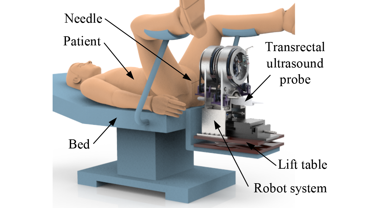
In this paper, an 8-DOF robot system is designed for ultrasound-imaging-guided prostate percutaneous intervention, and the scenario is shown in Fig. 1. The patient is in a lithotomy position, and the robot system uses the space between the two legs. The robot system is designed to realize hands-free activities of probe manipulation, needle positioning, and needle insertion. The decoupled motions allow the physician carry out more complicated and flexible activities. To simplify the robot system structure, the horizontal and vertical adjustments of the robot system base are accomplished by a manual lift table. As shown in Fig. 1, the robot system base is fixed on a lift table. By adjusting vertical and horizontal positions of the lift table, the ultrasound probe axis is aligned with the patient’s anus. Then, the lift table is locked on the bed, and the lift table and the robot system base are kept fixed during the whole scanning and intervention process.

Fig.1 Configuration of 8-DOF robot system for ultrasound-guided prostate percutaneous intervention.

Full size|PPT slide

The robot structure is shown in Fig. 2. The robot dimension is 254 mm × 420 mm × 488 mm (the length 420 mm is measured excluding the two devices because the total length changes as the needle and the probe move). The robot contains a 2-DOF structure for ultrasound probe movement, as shown in Fig. 2(a), a 4-DOF parallel structure for needle positioning, as shown in Fig. 2(b), and a 2-DOF structure for needle insertion, as shown in Fig. 2(c). The bases of the ultrasound probe manipulator and the needle positioning manipulator are both fixed on the lift table, as shown in Fig. 1.

Fig.2 Robot system including (a) 2-DOF ultrasound probe manipulator, (b) 4-DOF needle positioning manipulator, and (c) 2-DOF needle driver.

Full size|PPT slide

2.1 2-DOF ultrasound probe manipulator

The 2-DOF ultrasound probe manipulator is used to rotate and move the transrectal ultrasound probe along its axis, as shown in Fig. 3. The two DOFs can realize the motions needed for ultrasound probe scanning. Motors 1 and 2 are used to realize the rotation and the linear motion of the probe, respectively. A rubber block is wrapped around the probe for adjustment and locking. The rubber block is a quick-changing part that is easy to be sterilized.

Fig.3 2-DOF ultrasound probe manipulator structure.

Full size|PPT slide

2.2 4-DOF needle positioning manipulator

The 4-DOF needle positioning structure is used to orient and position the 2-DOF needle driver, as shown in Fig. 4. This part utilizes a parallel structure to increase rigidity and avoid collision between the moving parts and the patient. The structure mainly contains two similar stages assembled on the base, and each stage contains a scissor mechanism as end effector, as shown in Fig. 4(a).

Fig.4 4-DOF needle positioning manipulator: (a) two-stage structure, (b) single-stage structure, and (c) preload and positioning structure.

Full size|PPT slide

2.2.1 Single-stage structure and driving system

The single-stage structure is shown in Fig. 4(b) and mainly contains two separate transmission systems (labeled by purple and blue colors separately in the figure). Each transmission is composed of motor module, timing belt, and disc module. The motor module contains motor, relative encoder, reducer, coupler, small pulley, related shafts, and mounting parts (motor: DCX16L, planetary gearhead: GPX16, sensor: ENX16, Maxon, Switzerland). The disc module contains a large pulley, which is driven by timing belt transmission.

Bearings are used to position the rotating disc modules. As shown in Fig. 4(c), positioning slide bearing is used to change timing belt shape and avoid confliction between timing belt 2 and the base part. Small guide slots are reserved on the supporting board to allow position adjustments of the motor modules, such that pretightening force can be exerted on the timing belts. Two stages have the same transmission structures, where four motor modules are used to drive four rotating disc modules.

2.2.2 Scissor mechanism end effector

The two stages contain similar end effectors, and each end effector is a scissor mechanism formed by four hinged arms. Two arms are hinged to the two rotating disc modules of the same stage, as shown in Fig. 5(a). The relative motion between two hinged points impels the scissor mechanism end to extend or retract, as shown in Fig. 5(b). When two hinged points rotate together, the end trail can cover all the space inside the rotating disc.

Fig.5 Scissor mechanism assembly including (a) scissor mechanism installation and (b) motion principle.

Full size|PPT slide

The needle driver passes through the two scissor mechanism ends of the top and bottom stages. As shown in Fig. 6, the end structure of the bottom stage is a customized Hooke joint. This structure restricts axial rotation and sliding motion, but allows rotation along the two other axes. The end structure of the top stage is a centripetal joint bearing, where the needle driver passes through the central hole, and can rotate freely in all directions and slide along the needle driver axis. The structure design allows distance changing between the two end effectors when the needle driver moves.

Fig.6 Structures of two-stage scissor mechanism ends.

Full size|PPT slide

2.2.3 Position measurement devices

Limited by the mechanical structure, the absolute position of parallel structure is acquired by the combination of the relative encoder and the limit switch. The parallel structure contains four timing belt–pulley transmission. For each transmission, a relative encoder is assembled in motor module, and an optoelectronic switch (PM-L25, Panasonic, Japan) is assembled near the disc module, as shown in Fig. 7. A flag is mounted on the disc module, and the optoelectronic switch is mounted on the supporting board. To calibrate the system parameter, an optical tracking system is used, and the positions for spherically mounted retroreflectors (SMRs) are reserved on the rotating discs.

Fig.7 4-DOF needle positioning manipulator position measurement structure.

Full size|PPT slide

2.3 2-DOF needle driver

The 2-DOF needle driver realizes the rotation and the linear motion of the needle along its axis. The structure uses a compact design to decrease structure dimension and avoid overturning. As shown in Fig. 8, the needle driver passes through the top and bottom scissor mechanism ends. As the two ends are positioned, the pose of the needle driver is oriented. Fixture 1 is hinged to the Hooke joint of the bottom stage; Fixture 2 passes through the centripetal joint bearing of the top stage; and the two fixtures are fixed by screws.

Fig.8 Compact design of 2-DOF needle driver structure.

Full size|PPT slide

The needle driver contains two identical motor modules (motor: DCX10S, planetary gearhead: GPX10, sensor: ENX10, Maxon, Switzerland). For the linear joint, the mounting plate moves relative to Fixture 2 by gear rack pair transmission. For the rotary joint, the insert needle is fixed with a bevel gear; driven by motor module 2 and bevel gear pair transmission, the needle can realize self-rotation. To separate the needle and other parts of the needle driver, a sterilizable long tube is applied as a needle guide. The needle guide is fixed at the end of Fixture 1 by screws, in case of undesired hurts caused by needle guide motions during positioning.

Same as the 4-DOF needle positioning manipulator, the 2-DOF needle driver uses the combination of relative encoder and limit switch–flag pair to acquire joint absolute position. As shown in Fig. 9, the two limit switches are assembled on Fixture 2 and the mounting plate, and flags are assembled on the moving parts in each joint.

Fig.9 2-DOF needle driver position measurement structure.

Full size|PPT slide

To sum up, the 8-DOF robot system is designed for ultrasound probe manipulation, needle positioning, and insertion. In the robot system, the 2-DOF probe manipulator is a reliable structure for probe axial rotation and insertion. The other 6-DOF structure is placed above the probe manipulator to decrease the system volume. The 4-DOF parallel structure can realize needle positioning without motor or cable movement. This design increases system rigidity and decreases the potential risk of undesired collision between the robot body and the patient. The 2-DOF needle insertion structure uses compact distributions to reduce overturning torque.

3 Kinematic calibration and parameter identification

In the robot system, the 2-DOF probe manipulator and the 2-DOF needle driver are serial structures with coaxial linear and rotation joints, and calibration can be accomplished by the combination of the DH method and the least squares algorithm. The 4-DOF needle positioning manipulator is a parallel structure and needs an effective method to calibrate error parameters. In this paper, the structure model is built first, and a calibration method for the 4-DOF needle positioning manipulator is carried out.

3.1 Forward kinematic model and modification

3.1.1 Robot kinematic model

The 4-DOF needle positioning manipulator contains two stages, and the geometric model of one stage is shown in Fig. 10(a). The origin of the base coordinate system is placed at the hinge circle center. The scissor arms are labeled as AD, BE, DT, and ET. A and B are hinged points, and arms AD and BE are hinged at point C. DT and ET are hinged at end point T.

Fig.10 Geometrical relationships of (a) single-stage scissor mechanism and (b) two-stage scissor mechanisms.

Full size|PPT slide

The inputs of kinematics are the rotating angles of scissor mechanism arms. The geometrical relationships show that the position of end point T satisfies the following equation:

(1)\begin{array}{rl}{\mathit{P}}_T=& f\left({\theta }_1,{\theta }_2,d_1,d_2,r\right)=\frac{r}{2}\left[\begin{array}{c}\cos {\theta }_1+\cos {\theta }_2\\ \sin {\theta }_1+\sin {\theta }_2\end{array}\right]+\left(d_1+2d_2\right)\\ & \cdot \frac{\sqrt{1-{\displaystyle \frac{r^2}{2d_1^2}}\left(1-\cos \left({\theta }_2-{\theta }_1\right)\right)}}{\sqrt{2\left(1-\cos \left({\theta }_2-{\theta }_1\right)\right)}}\left[\begin{array}{c}-\left(\sin {\theta }_2-\sin {\theta }_1\right)\\ \cos {\theta }_2-\cos {\theta }_1\end{array}\right],\end{array}

where P_T is the position vector of point T, f(·) is the position function of vector P_T, θ₁ and θ₂ are the rotating angles of points A and B, respectively, d₁ and d₂ are the lengths of the scissor mechanism arms, l_AC = l_BC = d₁, l_CD = l_DT = l_TE = l_EC = d₂, and r is the radius of the circle where the hinged points slide.

In Fig. 10(b), the geometric model of the two-stage scissor mechanism is presented, and both stages share the same models. The coordinate system is placed above the top stage, and the xOy plane is defined by the SMR assembly plane. The subscripts t, b and f indicate that the parameters belong to top stage, bottom stage and needle tip, respectively. Assuming a needle passes through top end T₁ and bottom end T₂, the needle tip is denoted as T_f, and then the position vector of needle tip T_f can be calculated as follows:

(2){\mathit{P}}_{T_{\text{f}}}={\mathit{P}}_{T_{\text{2}}}+\frac{{\mathit{P}}_{T_{\text{2}}}-{\mathit{P}}_{T_{\text{1}}}}{\Vert {\mathit{P}}_{T_{\text{2}}}-{\mathit{P}}_{T_{\text{1}}}\Vert }l,

where {\mathit{P}}_{T_i} is the position vector of point T_i, i ∈{1, 2, f}, and l is the distance between needle end T_f and hinged point T₂.

3.1.2 Robot kinematic model modification

To calibrate the system kinematic parameters, the kinematic model is reconstructed with manufacturing and assembly errors.

Single stages are considered first. The values of θ₁ and θ₂ are obtained by the sum of relative encoder readings and home positions. The home position can be obtained from the computer aided design model, and a more precise value should be identified by calibration. To present the manufacturing and assembly errors on the system precision, these error items are integrated into the single-stage kinematic model Eq. (1), as shown in the following equation:

(3)\begin{array}{rl}{\mathit{p}}_T^{\ast }=& f\left({\theta }_1+\delta {\theta }_1,{\theta }_2+\delta {\theta }_2,d_1+\delta d_1,d_2+\delta d_2,r+\delta r\right)+\left[\begin{array}{c}\delta x\\ \delta y\end{array}\right]\\ =& f^{\text{*}}\left({\theta }_1,{\theta }_2,\delta {\theta }_1,\delta {\theta }_2,\delta d_1,\delta d_2,\delta r,\delta x,\delta y\right),\end{array}

where {\mathit{P}}_T^{\text{*}} is the modified position vector of point T, f^{\text{*}}(·) is the modified position function of vector {\mathit{P}}_T^{\text{*}}, d₁, d₂, r, θ₁, θ₂, and f(·) have same meanings as in Eq. (1), δj is the error of corresponding variable, where j∈{d₁, d₂, r, θ₁, θ₂}, and δx and δy are disc center errors with respect to the system base coordinate. For the single stage, seven error parameters, namely, {δθ₁, δθ₂, δd₁, δd₂, δr, δx, δy} need to be calibrated.

When the two stages are assembled as in Fig. 10(b), extra errors are introduced to the system. The errors mainly include position and coaxial errors, and the needle end tip equation is modified as Eq. (4):

(4)\{\begin{array}{c}{\mathit{P}}_{T_1}^{\text{*}}\text{=}\left[\begin{array}{c}{f_{\text{t}}}^{\text{*}}\left({\theta }_{\text{t}1},{\theta }_{\text{t}2}\right)\\ {\mathit{\text{z}}}_{\text{t}}\end{array}\right]+\left[\begin{array}{c}\delta x_{\mathrm{t}}\\ \delta y_{\mathrm{t}}\\ \delta {\mathit{\text{z}}}_{\mathrm{t}}\end{array}\right],\\ {\mathit{P}}_{T_2}^{\text{*}}\text{=}\left[\begin{array}{c}{f_{\text{b}}}^{\text{*}}\left({\theta }_{\text{b}1},{\theta }_{\text{b}2}\right)\\ {\mathit{\text{z}}}_{\text{b}}\end{array}\right]+\left[\begin{array}{c}\delta x_{\mathrm{b}}\\ \delta y_{\mathrm{b}}\\ \delta {\mathit{\text{z}}}_{\mathrm{b}}\end{array}\right],\\ {\mathit{P}}_{T_{\text{f}}}^{\text{*}}={\mathit{P}}_{T_2}^{\text{*}}+\frac{{\mathit{P}}_{T_2}^{\text{*}}-{\mathit{P}}_{T_1}^{\text{*}}}{\Vert {\mathit{P}}_{T_2}^{\text{*}}-{\mathit{P}}_{T_1}^{\text{*}}\Vert }l,\end{array}

where {\mathit{P}}_{T_i}^{\text{*}} is the modified position vector of point T_i, i∈{1, 2, f}, f_{\text{t}}^{\text{*}}(\cdot ) and f_{\text{b}}^{\text{*}} (\cdot ) are the modified kinematic position functions of the top and bottom stage end vectors, respectively, {θ_t1, θ_t2} and {θ_b1, θ_b2} are the angle inputs for the top and bottom stages, respectively, and {δx_t, δy_t, δz_t} and {δx_b, δy_b, δz_b} are the scissor mechanism end position errors of the top and bottom stages, respectively. The distances between the xOy plane and top stage, bottom stage, and needle tip are denoted as z_t, z_b, and z_f, respectively. ||·|| is the norm of the corresponding vector. The parameters for two-stage system calibration are {δx_t, δy_t, δz_t, δx_b, δy_b, δz_b}.

3.2 Robot calibration with PSO based on informative value

3.2.1 Calibration overview

Calibration is applied to identify the unknown parameters in the modified kinematic models. Considering the nonlinearity of the parallel robot kinematic model, PSO is applied in this paper during parameter identification for its rapid calculation speed. However, during iteration, the PSO method is not under a real-time supervision, and the final results may be converted to unreasonable values. To solve this problem, the PSO method is expected to be combined with the parameter characteristics.

In this paper, the informative value is combined with the PSO, and a method named InfoPSO is proposed. The informative value is a nondimensional value that reflects the discernibility of each parameter, and the calculation detail is explained in Section 3.2.3.

The scheme of InfoPSO is shown in Fig. 11. Each single-stage kinematic model has seven parameters that need to be identified. Combining the informative values with PSO, the modified single-stage model can be acquired. Based on the modified top-stage model, bottom-stage model, informative values of two-stage model parameters, and PSO, the modified two-stage model can be acquired.

Fig.11 Scheme diagram of 4-DOF parallel structure.

Full size|PPT slide

3.2.2 PSO approach review

PSO is a group intelligence optimization algorithm imitating the process of birds searching for food based on information exchange. The main process is as follows:

a) Generate primary particles. In the D-dimension solution space, N particles are defined randomly, and each particle is a candidate solution for the problem. The particle swarm is \left\{{\mathit{P}}_1^0,{\mathit{P}}_2^0,...,{\mathit{P}}_i^0,...,{\mathit{P}}_N^0\right\}. For each particle, {\mathit{P}}_i^0=\left\{x_{i1}^0,x_{i2}^0,...,x_{ij}^0,...,x_{iD}^0\right\}, where “0” represents the first generation, i is the particle number, and x_{ij}^0 means the value of ith particle at jth dimension. The primary velocity of the ith particle is defined as {\mathit{V}}_i^0=\{v_{i1}^0,v_{i2}^0, ...,v_{ij}^0,...,v_{iD}^0\}.

b) Calculate individual and swarm fitness values. For the searching, the fitness values are used to guide the particle swarm finding the target. The swarm fitness value gbest^k is the particle that fits the objective function best in the particle swarm until the current generation k; for each particle i, the value fits the objective function best in its history is the individual fitness value {\mathit{p}\mathit{b}\mathit{e}\mathit{s}\mathit{t}}_i^k.

c) Update the particle swarm velocity. Referring to the fitness values of individual and swarm, the particle values are updated by corresponding velocity. For the ith particle, the velocity is

(5){\mathit{V}}_i^{k+1}= \omega \times {\mathit{V}}_i^k+c_1\times \mu \times \left({\mathit{p}\mathit{b}\mathit{e}\mathit{s}\mathit{t}}_i^k-{\mathit{P}}_i^k\right)+c_2\times \eta \times \left(\mathit{g}\mathit{b}\mathit{e}\mathit{s}{t}^k-{\mathit{P}}_i^k\right),

where \omega is the inertia weight reflecting the influence of current velocity, c₁ and c₂ are particles’ cognitive and social factors, respectively, and μ and η are random values in (0, 1). The velocity of dimension j is restricted by a maximum velocity v_{max}^j. If velocity v_{ij}^{k+1}> v_{max}^j, then v_{ij}^{k+1}\text{=}{v}_{max}^j; if , then v_{ij}^{k+1}\text{=}-v_{max}^j.

d) Update particle value. Based on the current value and updated velocity, the next generation of particles can be obtained as

(6){\mathit{P}}_i^{k+1}= {\mathit{P}}_i^k+ {\mathit{V}}_i^{k+1}.

e) Update the fitness values. The current fitness of each particle in the new generation is calculated. For each particle, the individual fitness value is replaced with the new fitness value if the latter is better. Among all the fitness values in the current generation, the best fitness value is searched and compared with the swarm fitness, and the better one is selected as the swarm fitness value. Steps c)–e) are repeated until the swarm fitness value satisfies the task requirement or the cycle counter reaches the maximum value.

3.2.3 Informative value calculation

In PSO, particles are randomly generated, and each particle is a candidate for kinematic modeling. During searching, the fitness value is the only evaluation standard, and all the parameters are identified simultaneously. Though a large difference exists between two particle candidates, the fitness values may locate close to each other. The phenomenon results from that different parameters have varied influence rates or different “parameter discernibility.” The changes led by parameters with less discernibility may be omitted by those changes led by parameters with more discernibility. To realize the identification accurately, parameters with different discernibility magnitude orders should be identified separately. The derivation of parameter discernibility is shown in Appendix A. In general, the derivation includes two steps: First, the gradients of all parameters belonging to {δθ₁, δθ₂, δd₁, δd₂, δr, δx, δy} are calculated; then, the high-order terms in the gradient are neglected for a convenient calculation. When high-order terms are ignored, the constant term coefficient is remarkable enough to show the discernibility of one parameter because the identified error parameters are all near 0. The constant term is defined as the “informative value” to reflect the parameter discernibility.

The informative values of all the parameters are shown in Table A1. For each parameter, the x and y components are functions of θ₁ and θ₂, that is, the informative values of the error parameters may vary as the function inputs change. In theory, the definition domain of θ₁ and θ₂ are (−180°, 180°). Considering the restriction of parallel structure, θ₁ changes freely in (−180°, 180°), whereas θ₂ is limited in the range of (θ₁+30°, θ₁+50°). These input restrictions hold for all parameter informative value calculations.

The informative values of all the parameters are illustrated in Fig. 12. The informative values are labelled as I(·) for short, and for each parameter, the informative value contains components on the x and y axis and both are shown in Fig. 12. For a clear comparation, the maximum informative values of the parameters are listed in Table 1.

Tab.1 Maximum informative value of error parameters in modified forward kinematics

Error parameter	Maximum informative value
δθ1	269.1
δθ2	269.1
δd1	9.1
δd2	1.6
δr	4.9
δx	(Constant) 1.0
δy	(Constant) 1.0

Fig.12 Informative values of error parameters in the modified kinematic model (θ₁ ∈ (−180°, 180°), θ₂ ∈ (θ₁+30°, θ₁+50°)): (a) informative value of δθ₁ and δθ₂, (b) informative value of δd₁ and δr, and (c) informative value of δd₂, δx, and δy.

Full size|PPT slide

Figure 12 and Table 1 show that the informative values vary greatly. The maximum values of I(δθ₁) and I(δθ₂) are much larger than the other parameters, which means the value fluctuations of δθ₁ and δθ₂ greatly influence the values of other parameters during identification. The informative values of δd₁ and δr are also larger than δd₂, δx, and δy. If all the parameters are explored simultaneously, the parameters with larger informative values harmfully affect other parameter identification processes. The optimization should consider informative values and carry out the process stepwise.

As shown in Eq. (4), the two-stage system contains offset parameters {δx_t, δy_t, δz_t, δx_b, δy_b, δz_b}, where {δx_t, δy_t, δz_t} and {δx_b, δy_b, δz_b} are offsets for the top end and the bottom end, respectively. The error parameters are homogenous in Eq. (4), and their informative values are all constantly 1.0 (similar to δx and δy in Fig. 12). These six parameters can be identified in a single-step process.

3.2.4 PSO based on informative value

The 4-DOF needle positioning manipulator calibration is carried out, as shown in Fig. 13, and the two single stages are calibrated separately first. In this paper, InfoPSO is applied as the identification method. The informative values prove that different parameters have distinct discernibility, and the seven parameters are classified into three groups according to the magnitude orders of informative values, namely, {δθ₁, δθ₂}, {δd₁, δr}, and {δd₂, δx, δy}. Three groups of parameters are identified in a three-step identification sequence. When one group of parameters is identified, the other parameters are set to be 0 (not identified yet) or result values (already identified). The constants r, d₁, and d₂ use designed values. θ₁ and θ₂ are obtained by the sum of theoretical home positions and real-time readings of relative encoders. The real end effector position P_T is collected for each pair of {θ₁, θ₂}, and M groups of {θ₁, θ₂, P_T} are collected and applied for PSO. The fitness value ε for each particle is defined as the quadratic criterion error:

Fig.13 Scheme of 4-DOF positioning manipulator calibration by InfoPSO.

Full size|PPT slide

(7)\epsilon =\frac{1}{M}\sum _{i=1}^M{\Vert {\mathit{P}}_T^i-f^{\text{*}}\left({\theta }_1^i,{\theta }_2^i,\delta {\theta }_1,\delta {\theta }_2,\delta d_1,\delta d_2,\delta r,\delta x,\delta y\right)\Vert }^2,

where f^{\text{*}}(·) is the modified model as Eq. (3).

When one group of parameters changes, other parameters may be disturbed because of parameter interaction. Thus, a repetition of the three-step identification is needed until all of the parameters remain unchanged.

After the single stages are identified, the two-stage system is assembled, and {δx_t, δy_t, δz_t, δx_b, δy_b, δz_b} are parameters for identification. Equation (4) shows that the six parameters share the same informative value (all constantly 1.0); thus, the identification can be finished by one-step PSO. For one group of {θ_t1, θ_t2, θ_b1, θ_b2}, the needle driver passing T₁T₂ is oriented, and the needle tip reaches {\mathit{P}}_{T_{\text{f}}}, as shown in Fig. 10(b). N groups of {θ_t1, θ_t2, θ_b1, θ_b2, {\mathit{P}}_{T_2}, {\mathit{P}}_{T_{\text{f}}}} are collected for PSO, and then the fitness value for one particle is defined as

(8)\begin{array}{rl}\epsilon =& \frac{1}{N}({\alpha }_1\sum _{i=1}^N{\Vert {\mathit{P}}_{T_{\text{f}}}^i-{\mathit{P}}_{T_{\text{f}}}^{\ast }\left({\theta }_{\text{t1}}^i,{\theta }_{\text{t}2}^i,{\theta }_{\text{b}1}^i,{\theta }_{\text{b}2}^i\right)\Vert }^2\\ & +{\alpha }_2\sum _{j=1}^N{\Vert {\mathit{P}}_{T_2}^j-{\mathit{P}}_{T_2}^{\ast }\left({\theta }_{\text{t}1}^j,{\theta }_{\text{t}2}^j,{\theta }_{\text{b}1}^j,{\theta }_{\text{b}2}^j\right)\Vert }^2),\end{array}

where {\mathit{P}}_{T_{\text{f}}}^{\ast } and {\mathit{P}}_{T_2}^{\ast } are defined as Eq. (4), {\mathit{P}}_{T_2} is approximately regarded as the insertion point, α₁ and α₂ are the weight factors of target accuracy and insertion point accuracy, respectively, and α₁ + α₂ = 1.

4 Experiment

The robot system is assembled, and the platform is built for calibration, as shown in Fig. 14. The motors are driven by actuators (G-SOLWHI2.5/100EE, Elmo), and the controller is an industrial personal computer from Beckhoff. To collect position data, an optical tracking system is used (AT960, Leica, Switzerland).

Fig.14 Experimental platform of 8-DOF percutaneous intervention robot calibration.

Full size|PPT slide

4.1 Single-stage structure calibration

First, the two stages are analyzed separately. A single stage is assembled, and an equivalent weight is adhered to the top stage end effector to simulate the force exerted by the needle driver assembly. After the system powers on, the two rotating discs rotate together until both hit the limit switches. Then, the home positions are determined according to the limit switch positions and the predefined offsets of each joint. The end effector control is based on one-stage kinematics, and optical tracking system is used to collect position data of mechanism end, as shown in Fig. 15(a). Twelve traces are selected uniformly, and the positions of eight points are collected along each trace, as shown in Fig. 15(b). The process is repeated three times, and 288 groups of data are collected. The collected data are applied to the InfoPSO in Fig. 13, and the single-stage parameter errors can be identified.

Fig.15 Single-stage position accuracy experiment: (a) coordinate system position, (b) end point position selection.

Full size|PPT slide

The positions of targeting experiments at the top and bottom stages are shown in Fig. 16. The single-stage parameter identification results calculated by the traditional PSO and InfoPSO are shown in Tables 2 and 3, and the designed values are listed. To compare the results intuitively, the square root of the quadratic criterion error in Eq. (7) is defined as “average error” to judge the results. The average error is focused on the mechanical error, and no ultrasound image error is considered. Thus, the data collected by the optical tracking system can be used to calibrate the kinematic parameters.

Tab.2 Parameter identification results of top-stage structure

Method	δθ1/rad	δθ2/rad	δr/mm	δd1/mm	δd2/mm	δx/mm	δy/mm	Average error/mm
Initial value	0	0	0	0	0	0	0	2.778
InfoPSO	−0.012	−0.015	1.466	0.966	−0.009	0.355	−1.752	1.499
Traditional PSO	−0.011	−0.017	59.296	35.221	12.157	0.251	−1.777	1.395

Tab.3 Parameter identification results of bottom-stage structure

Method	δθ1/rad	δθ2/rad	δr/mm	δd1/mm	δd2/mm	δx/mm	δy/mm	Average error/mm
Initial value	0	0	0	0	0	0	0	1.543
InfoPSO	0.002	−0.007	2.193	1.395	0.001	0.426	0.130	0.975
Traditional PSO	0.002	−0.008	48.382	28.037	10.239	0.351	0.112	0.899

Fig.16 Single-stage targeting results: (a) top stage position collection, (b) bottom stage position collection.

Full size|PPT slide

In Tables 2 and 3, initially, the parameters are all set to be 0, and the average errors are 2.778 and 1.543 mm for the top stage and the bottom stage, respectively. By applying InfoPSO, the average errors are reduced to 1.499 and 0.975 mm for the top stage and the bottom stage, respectively. The traditional PSO and InfoPSO contain similar results for δθ₁ and δθ₂ (parameters with high informative values), whereas the other parameters are remarkably different. Though the average error of traditional PSO is smaller than that of InfoPSO, the length errors δr, δd₁, and δd₂ identified by the traditional PSO are larger than 10 mm. For example, the δr of the top stage is approximately 59 mm, which means that the manufactured disc radius is 59 mm larger than the designed model. The unreasonable results suggest that the identified results of the traditional PSO are only fit for the collected data group. If another data group is collected in additional experiments, the large error parameters may lead to an unreliable end position. As an alternative choice, the results of InfoPSO are more trustworthy and applicable for robot kinematics. The reasonability is also proven by the fact that the same manufacturing errors of the two stages are close to one another. The average error of the top stage is larger than that of the bottom one because the added weight is exerted on the top stage (simulating the needle driver gravity), and the force leads to a larger deviation to the end effector position.

4.2 Two-stage structure calibration

The two stages and the needle driver are assembled together. As mentioned above, six parameters {δx_t, δy_t, δz_t, δx_b, δy_b, δz_b} are identified simultaneously. The coordinate system is built above the top stage, as shown in Fig. 10, and 21 points are selected uniformly from both stages, as shown in Fig. 17. For each point from the top stage, the neighbor points in the bottom stage are selected as point pairs. A total of 141 groups of point pairs are selected. For each pair, the needle driver is oriented by scissor mechanism end effectors, and {θ_t1, θ_t2, θ_b1, θ_b2, {\mathit{P}}_{T_2}, {\mathit{P}}_{T_{\text{f}}}} are collected. As in Eq. (8), the fitness value is defined as the average of the quadratic criterion error at the bottom stage point (near body insertion point) and the needle tip point.

Fig.17 Coordinate system distribution and needle driver orientation selection for two-stage targeting accuracy experiment.

Full size|PPT slide

The identified parameters and their designed values are listed in Table 4. The average error is a judgement of accuracy at the insertion point and the needle tip, and is defined as the square root of ε in Eq. (8). The weight factors of target accuracy α₁ = α₂ = 0.5. The results are reasonable and show that the average error is reduced from 3.198 to 1.594 mm.

Tab.4 Parameter identification results of two-stage structure

Value source	zt/mm	zb/mm	δxt/mm	δyt/mm	δxb/mm	δyb/mm	Average error/mm
Designed value	−25.000	−130.000	0	0	0	0	3.198
Identified Value	−27.150	−134.850	0.084	0.073	0.028	0.034	1.594

To sum up, the parameters for kinematics modification are listed in Table 5. δθ₁ and δθ₂ are disc module offsets based on theoretical home positions, r^{\ast } is the modified hinged point circle radius, d_1^{\ast } and d_2^{\ast } are the modified scissor mechanism arm lengths, δx and δy are the disc module center errors with respect to the system coordinate system, and {\mathit{\text{z}}}^{\ast } is the z component of the end effector position with respect to the system coordinate system. All the modified parameters are substituted into system kinematics, and a verification experiment is carried out as follows.

Tab.5 Parameters used for 4-DOF positioning manipulator kinematics

Stage information	δθ1/rad	δθ2/rad	r^{\ast }/mm	d_1^{\ast }/mm	d_2^{\ast }/mm	δx/mm	δy/mm	{\mathit{\text{z}}}^{\ast }/mm
Top stage	−0.012	−0.015	66+1.466	30+0.966	45−0.009	0.4381	−1.6791	−27.150
Bottom stage	0.002	−0.007	66+2.193	30+1.395	45+0.001	0.4535	0.1635	−134.850

4.3 System verification experiment

The identified parameters in Table 5 are applied to modify the kinematic model, and the two-stage experiments in Section 4.2 are repeated. The target positions at the top and bottom stages are selected uniformly and different from previous configurations. The results are compared at z = −140 mm (near the insertion point) and z = −200 mm (near the needle tip), as shown in Fig. 18. The black and red points show the distribution of results calculated by original kinematics and modified kinematics, respectively, in contrast to the collected points with blue color. In Fig. 18(b), grey circles are applied to indicate the data groups.

Fig.18 Comparison of targeting results between calculated and experiment positions at insertion and target depth: (a) z = −140 mm, (b) z = −200 mm. Black: initial kinematics; red: modified kinematics; blue: collected positions.

Full size|PPT slide

The figures show that the points obtained by modified kinematics (red) are located closer to the measured data (blue). In Fig. 18(a), the average error of original kinematics is approximately 1.497 mm, and modified kinematics shows an error of 0.963 mm. In Fig. 18(b), the average error of the original kinematics is approximately 2.654 mm, and modified kinematics shows an error of 1.846 mm. The error of the needle tip is reduced by 43.8%, which proves that the kinematic modification substantially improves accuracy. Compared with similar robots for prostate percutaneous intervention [34], reaching a targeting accuracy smaller than 2 mm is acceptable for the parallel structure prototype.

For a further comparison, the boxplots of the system targeting experiments are shown in Fig. 19. The x axis shows the distance between the collected positions and the hinged circle center. At z = −140 mm, the data are distributed near the selected positions of the bottom stage, and the points are classified according to the positions at the bottom stage. At z = −200 mm, the data are distributed more uniformly, and the points are classified into different distance ranges such as 10–20 mm. The y axis shows the distances between the calculation positions and the corresponding collected positions. In general, the average values and the standard deviations for the modified kinematics are decreased, which means that compared with the original kinematic model, the results calculated by the modified kinematic model have less variability and are better in accordance with the real condition. Comparing Fig. 19(b) with Fig. 19(a) shows that the results of the bottom stage are better than those of the top stages because the needle driver exerts more force on the top stage, and gravity error (which is not considered in this paper) has more influence on the top stage, especially near the hinged circle center.

Fig.19 Boxplot of system targeting experiment at insertion and target depth: (a) z = −140 mm, (b) z = −200 mm.

Full size|PPT slide

5 Conclusions

In this paper, an 8-DOF ultrasound-guided prostate percutaneous intervention robot system is designed to assist physicians in realizing hands-free ultrasound probe scanning, needle pose adjustment, and needle insertion. The structure is novel with high rigidity and compactness, and can help the probe and the needle realize the required movements as well as decrease the potential risk of confliction between the robot body and the patient. To calibrate the parallel structure and identify the error parameters with different discernibility, InfoPSO is proposed. In stepwise InfoPSO, the single- and two-stage parameters are identified to modify the kinematics. The targeting experiments show that the identified parameters for the kinematic model modification are reasonable. By applying the modified kinematic model, the parallel structure can reach average errors of 0.963 and 1.846 mm at needle insert position and target position, respectively. The error of the needle tip is reduced by 43.8% compared with that of the initial kinematic model. The improvement proves that the calibration method is practicable, and InfoPSO provides an available, trustworthy solution for robot kinematic parameter identification.

6 Appendices

Appendix A Kinematic parameter discernibility analysis for single-stage parallel structure

The geometric model of the single-stage parallel structure is shown in Fig. 10(a), and the position vector of end point P_T is presented as Eq. (1). Considering the error parameters {δθ₁, δθ₂, δd₁, δd₂, δr, δx, δy}, the revised single-stage kinematic equation is presented as Eq. (3). Without loss of generality, δθ₁ is taken as an example. The partial derivative with respect to δθ₁ is taken, the six other errors {δθ₂, δd₁, δd₂, δr, δx, δy} are set to be 0 for calculation simplification. Taylor series expansion is applied to the partial derivative at point δθ₁ = 0.

When high-order terms are ignored, the constant term coefficient is remarkable enough to reflect the influence rate of parameter δθ₁ in calculating end position vector P_T because the identified error parameters are all near 0. As explained in the paper, the constant term is the discernibility of the respective parameter or called informative value, which is denoted as I(δθ₁). The calculation is repeated, and the informative value for all parameters can be acquired, as shown in Table A1. The x and y components of one parameter are shown separately.

Table A1 Informative values of error parameters in modified forward kinematics

Parameter	Component	Informative value
δα1	x	\begin{array}{rl}& [16\left(d_1+2d_2\right)\left(2\left(d_1^2-r^2\right)\mathrm{c}\mathrm{o}\mathrm{s}{\theta }_1+r^2\mathrm{c}\mathrm{o}\mathrm{s}\left(2{\theta }_1-{\theta }_2\right)\right)-\left(\text{2}{d}_1^3+4d_1^2{d}_2-d_1{r}^2-2d_2{r}^2\right)\mathrm{c}\mathrm{o}\mathrm{s}{\theta }_2\\ & -2d_1^{2}r\sqrt{1-\mathrm{c}\mathrm{o}\mathrm{s}\left({\theta }_1-{\theta }_2\right)}\sqrt{2\text{+}\frac{r^2\left(\mathrm{c}\mathrm{o}\mathrm{s}\left({\theta }_1-{\theta }_2\right)-1\right)}{d_1^2}}\mathrm{s}\mathrm{i}\mathrm{n}{\theta }_1\text{Bigggr}]16{\mathrm{s}\mathrm{i}\mathrm{n}}^2\left(\frac{{\theta }_1-{\theta }_2}{2}\right)\\ & /\left(2d_1^2{\left(1-\mathrm{c}\mathrm{o}\mathrm{s}\left({\theta }_1-{\theta }_2\right)\right)}^{\frac{3}{2}}\sqrt{2\text{+}\frac{r^2\left(\mathrm{c}\mathrm{o}\mathrm{s}\left({\theta }_1-{\theta }_2\right)-1\right)}{d_1^2}}\right)\end{array}
	y	\begin{array}{rl}& {\mathrm{s}\mathrm{i}\mathrm{n}}^2\left(\frac{{\theta }_1-{\theta }_2}{2}\right)[152d_1^{2}r\mathrm{c}\mathrm{o}\mathrm{s}{\theta }_1\sqrt{1-\mathrm{c}\mathrm{o}\mathrm{s}\left({\theta }_1-{\theta }_2\right)}\sqrt{2\text{+}\frac{r^2\left(\mathrm{c}\mathrm{o}\mathrm{s}\left({\theta }_1-{\theta }_2\right)-1\right)}{d_1^2}}+(d_1+2d_2)(2\left(d_1^2-r^2\right)\mathrm{s}\mathrm{i}\mathrm{n}{\theta }_1\\ & +r^2\mathrm{s}\mathrm{i}\mathrm{n}(2{\theta }_1-{\theta }_2)+\left(r^2-2d_1^2\right)\mathrm{s}\mathrm{i}\mathrm{n}{\theta }_2)]15/\left(2d_1^2{\left(1-\mathrm{c}\mathrm{o}\mathrm{s}\left({\theta }_1-{\theta }_2\right)\right)}^{\frac{3}{2}}\sqrt{2\text{+}\frac{r^2\left(\mathrm{c}\mathrm{o}\mathrm{s}\left({\theta }_1-{\theta }_2\right)-1\right)}{d_1^2}}\right)\end{array}
δα2	x	\begin{array}{rl}& -{\mathrm{s}\mathrm{i}\mathrm{n}}^2\left(\frac{{\theta }_1-{\theta }_2}{2}\right)[15\left(d_1+2d_2\right)\left(-\left(2d_1^2-r^2\right)\mathrm{c}\mathrm{o}\mathrm{s}{\theta }_1-r^2\mathrm{c}\mathrm{o}\mathrm{s}\left({\theta }_1-2{\theta }_2\right)\right)+\left(2d_1^3+4d_1^2{d}_2-2d_1{r}^2-4d_2{r}^2\right)\mathrm{c}\mathrm{o}\mathrm{s}{\theta }_2\\ & +2d_1^{2}r\sqrt{1-\mathrm{c}\mathrm{o}\mathrm{s}\left({\theta }_1-{\theta }_2\right)}\sqrt{2\text{+}\frac{r^2\left(\mathrm{c}\mathrm{o}\mathrm{s}\left({\theta }_1-{\theta }_2\right)-1\right)}{d_1^2}}\mathrm{s}\mathrm{i}\mathrm{n}{\theta }_2]15/\left(2d_1^2{\left(1-\mathrm{c}\mathrm{o}\mathrm{s}\left({\theta }_1-{\theta }_2\right)\right)}^{\frac{3}{2}}\sqrt{2\text{+}\frac{r^2\left(\mathrm{c}\mathrm{o}\mathrm{s}\left({\theta }_1-{\theta }_2\right)-1\right)}{d_1^2}}\right)\end{array}
	y	\begin{array}{rl}& {\mathrm{s}\mathrm{i}\mathrm{n}}^2\left(\frac{{\theta }_1-{\theta }_2}{2}\right)[152d_1^{2}r\mathrm{c}\mathrm{o}\mathrm{s}{\theta }_2\sqrt{1-\mathrm{c}\mathrm{o}\mathrm{s}\left({\theta }_1-{\theta }_2\right)}·\sqrt{2\text{+}\frac{r^2\left(\mathrm{c}\mathrm{o}\mathrm{s}\left({\theta }_1-{\theta }_2\right)-1\right)}{d_1^2}}\\ & +\left(d_1+2d_2\right)·\left(\left(2d_1^2-r^2\right)\mathrm{s}\mathrm{i}\mathrm{n}{\theta }_1+r^2\mathrm{s}\mathrm{i}\mathrm{n}\left({\theta }_1-2{\theta }_2\right)+2\left(r^2-d_1^2\right)\mathrm{s}\mathrm{i}\mathrm{n}{\theta }_2\right)]15\\ & /\left(2d_1^2{\left(1-\mathrm{c}\mathrm{o}\mathrm{s}\left({\theta }_1-{\theta }_2\right)\right)}^{\frac{3}{2}}\sqrt{2\text{+}\frac{r^2\left(\mathrm{c}\mathrm{o}\mathrm{s}\left({\theta }_1-{\theta }_2\right)-1\right)}{d_1^2}}\right)\end{array}
δl1	x	\left(d_1^3+d_2{r}^2-d_2{r}^2\cos \left({\theta }_1-{\theta }_2\right)\right)\left(\sin {\theta }_1-\sin {\theta }_2\right)/\left(d_1^3\sqrt{1-\cos \left({\theta }_1-{\theta }_2\right)}\sqrt{2+{\displaystyle \frac{r^2\left(\cos \left({\theta }_1-{\theta }_2\right)-1\right)}{d_1^2}}}\right)
	y	\begin{array}{l}-\left(d_1^3\text{+}{d}_2{r}^2-d_2{r}^2\mathrm{c}\mathrm{o}\mathrm{s}\left({\theta }_1-{\theta }_2\right)\right)\left(\mathrm{c}\mathrm{o}\mathrm{s}{\theta }_1-\mathrm{c}\mathrm{o}\mathrm{s}{\theta }_2\right)/\left(d_1^3\sqrt{1-\mathrm{c}\mathrm{o}\mathrm{s}\left({\theta }_1-{\theta }_2\right)}\sqrt{2\text{+}{\displaystyle \frac{r^2\left(\mathrm{c}\mathrm{o}\mathrm{s}\left({\theta }_1-{\theta }_2\right)-1\right)}{d_1^2}}}\right)\end{array}
δl2	x	\begin{array}{l}\sqrt{2\text{+}{\displaystyle \frac{r^2\left(\mathrm{c}\mathrm{o}\mathrm{s}\left({\theta }_1-{\theta }_2\right)-1\right)}{d_1^2}}}\left(\mathrm{s}\mathrm{i}\mathrm{n}{\theta }_1-\mathrm{s}\mathrm{i}\mathrm{n}{\theta }_2\right)/\sqrt{1-\mathrm{c}\mathrm{o}\mathrm{s}\left({\theta }_1-{\theta }_2\right)}\end{array}
	y	\begin{array}{l}\sqrt{2\text{+}{\displaystyle \frac{r^2\left(\mathrm{c}\mathrm{o}\mathrm{s}\left({\theta }_1-{\theta }_2\right)-1\right)}{d_1^2}}}\left(-\mathrm{c}\mathrm{o}\mathrm{s}{\theta }_1+\mathrm{c}\mathrm{o}\mathrm{s}{\theta }_2\right)/\sqrt{1-\mathrm{c}\mathrm{o}\mathrm{s}\left({\theta }_1-{\theta }_2\right)}\end{array}
δr	x	{\displaystyle \frac{1}{2}}\left(\mathrm{c}\mathrm{o}\mathrm{s}{\theta }_1+\mathrm{c}\mathrm{o}\mathrm{s}{\theta }_2+{\displaystyle \frac{\left(d_1+2d_2\right)r\sqrt{1-\mathrm{c}\mathrm{o}\mathrm{s}\left({\theta }_1-{\theta }_2\right)}\left(-\mathrm{s}\mathrm{i}\mathrm{n}{\theta }_1+\mathrm{s}\mathrm{i}\mathrm{n}{\theta }_2\right)}{d_1^2\sqrt{2\text{+}{\displaystyle \frac{r^2\left(\mathrm{c}\mathrm{o}\mathrm{s}\left({\theta }_1-{\theta }_2\right)-1\right)}{d_1^2}}}}}\right)
	y	{\displaystyle \frac{1}{2}}\left(\mathrm{s}\mathrm{i}\mathrm{n}{\theta }_1+\mathrm{s}\mathrm{i}\mathrm{n}{\theta }_2+{\displaystyle \frac{\left(d_1+2d_2\right)r\sqrt{1-\mathrm{c}\mathrm{o}\mathrm{s}\left({\theta }_1-{\theta }_2\right)}\left(\mathrm{c}\mathrm{o}\mathrm{s}{\theta }_1-\mathrm{c}\mathrm{o}\mathrm{s}{\theta }_2\right)}{\sqrt{2d_1^4\text{+}{r}^2{d}_1^2\left(\mathrm{c}\mathrm{o}\mathrm{s}\left({\theta }_1-{\theta }_2\right)-1\right)}}}\right)
δx	x	1
	y	0
δy	x	0
	y	1

Acknowledgements

This paper was supported by the Foundation for Innovative Research Groups of the National Natural Science Foundation of China (Grant No. 51521003), the National Natural Science Foundation of China (Grant No. 61803341), and the Self-Planned Task of State Key Laboratory of Robotics and System (Harbin Institute of Technology, China) (Grant No. SKLRS202009B). No conflicts of interest exist in this paper.

Open Access

This article is licensed under a Creative Commons Attribution 4.0 International License, which permits use, sharing, adaptation, distribution, and reproduction in any medium or format as long as appropriate credit is given to the original author(s) and source, a link to the Creative Commons license is provided, and indicate if changes were made.

The images or other third-party material in this article are included in the article’s Creative Commons license, unless indicated otherwise in a credit line to the material. If material is not included in the article’s Creative Commons license and your intended use is not permitted by statutory regulation or exceeds the permitted use, you will need to obtain permission directly from the copyright holder.

Visit http://creativecommons.org/licenses/by/4.0/ to view a copy of this license.

References

1 SiegelR L, MillerK D, JemalA. Cancer statistics. CA: A Cancer Journal for Clinicians, 2020, 70( 1): 7– 30

2 CarterH B. American Urological Association (AUA) Guideline on prostate cancer detection: process and rationale. BJU International, 2013, 112( 5): 543– 547

3 JiangS, YangY P, YangZ Y, ZhangZ, LiuS. Design and experiments of ultrasound image-guided multi-DOF robot system for brachytherapy. Transactions of Tianjin University, 2017, 23( 5): 479– 487

4 ThomasT L, VenkiteswaranV K, AnanthasureshG K, MisraS. Surgical applications of compliant mechanisms: a review. Journal of Mechanisms and Robotics, 2021, 13( 2): 020801–

5 UkimuraO, HiraharaN, FujiharaA, YamadaT, IwataT, KamoiK, OkiharaK, ItoH, NishimuraT, MikiT. Technique for a hybrid system of real-time transrectal ultrasound with preoperative magnetic resonance imaging in the guidance of targeted prostate biopsy. International Journal of Urology, 2010, 17( 10): 890– 893

6 SinghA K, KrueckerJ, XuS, GlossopN, GuionP, UllmanK, ChoykeP L, WoodB J. Initial clinical experience with real-time transrectal ultrasonography-magnetic resonance imaging fusion-guided prostate biopsy. BJU International, 2008, 101( 7): 841– 845

7 PoquetC, MozerP, VitraniM A, MorelG. An endorectal ultrasound probe comanipulator with hybrid actuation combining brakes and motors. IEEE/ASME Transactions on Mechatronics, 2015, 20( 1): 186– 196

8 LimS, JunC, ChangD, PetrisorD, HanM, StoianoviciD. Robotic transrectal ultrasound guided prostate biopsy. IEEE Transactions on Biomedical Engineering, 2019, 66( 9): 2527– 2537

9 SchlüterM, FürwegerC, SchlaeferA. Optimizing robot motion for robotic ultrasound-guided radiation therapy. Physics in Medicine and Biology, 2019, 64( 19): 195012–

10 YuX B, HeW, LiH Y, SunJ. Adaptive fuzzy full-state and output-feedback control for uncertain robots with output constraint. IEEE Transactions on Systems, Man, and Cybernetics: Systems, 2021, 51( 11): 6994– 7007

11 KongL Y, ChenG L, WangH, HuangG Y, ZhangD. Kinematic calibration of a 3-PRRU parallel manipulator based on the complete, minimal and continuous error model. Robotics and Computer-Integrated Manufacturing, 2021, 71 : 102158–

12 LiZ B, LiS, LuoX. An overview of calibration technology of industrial robots. IEEE/CAA Journal of Automatica Sinica, 2021, 8( 1): 23– 36

13 QuinteroH F, MejiaL A, Diaz-RodriguezM. End-effector positioning due to joint clearances: a comparison among three planar 2-DOF parallel manipulators. Journal of Mechanical Science and Technology, 2019, 33( 7): 3497– 3507

14 JiangZ H, ZhouW G, LiH, MoY, NiW C, HuangQ. A new kind of accurate calibration method for robotic kinematic parameters based on the extended Kalman and particle filter algorithm. IEEE Transactions on Industrial Electronics, 2018, 65( 4): 3337– 3345

15 GanY H, DuanJ J, DaiX Z. A calibration method of robot kinematic parameters by drawstring displacement sensor. International Journal of Advanced Robotic Systems, 2019, 16( 5): 1– 9

16 LiJ, YuL D, SunJ Q, XiaH J. A kinematic model for parallel-joint coordinate measuring machine. Journal of Mechanisms and Robotics, 2013, 5( 4): 044501–

17 HuangT, LiuH T, ChetwyndD G. Generalized Jacobian analysis of lower mobility manipulators. Mechanism and Machine Theory, 2011, 46( 6): 831– 844

18 TianW J, ShenZ Q, LvD P, YinF W. A systematic approach for accuracy design of lower-mobility parallel mechanism. Robotica, 2020, 38( 12): 2173– 2188

19 ZhangZ Y. A flexible new technique for camera calibration. IEEE Transactions on Pattern Analysis and Machine Intelligence, 2000, 22( 11): 1330– 1334

20 LiaoS H, ZengQ, EhmannK F, CaoJ. Parameter identification and nonparametric calibration of the tri-pyramid robot. IEEE/ASME Transactions on Mechatronics, 2020, 25( 5): 2309– 2317

21 DaneyD, PapegayY, MadelineB. Choosing measurement poses for robot calibration with the local convergence method and tabu search. The International Journal of Robotics Research, 2005, 24( 6): 501– 518

22 MaoC T, ChenZ W, LiS, ZhangX. Separable nonlinear least squares algorithm for robust kinematic calibration of serial robots. Journal of Intelligent & Robotic Systems, 2021, 101( 1): 2–

23 XuW Y, XuH D, LiuF K, TangY Y, WuZ, WangX J, WangJ, FengJ Q. Millimeter wave power monitoring in EAST ECRH system. IEEE Access: Practical Innovations, Open Solutions, 2016, 4 : 5809– 5817

24 KennedyJ, EberhartR. Particle swarm optimization. In: Proceedings of ICNN'95-International Conference on Neural Networks. Perth: IEEE, 1995, 1942– 1948

25 QiY, SunT, SongY M. Multi-objective optimization of parallel tracking mechanism considering parameter uncertainty. Journal of Mechanisms and Robotics, 2018, 10( 4): 041006–

26 FlockerF W, BravoR H. On global convergence in design optimization using the particle swarm optimization technique. Journal of Mechanical Design, 2016, 138( 8): 081402–

27 Gao G B, Liu F, San H J, Wu X, Wang W. Hybrid optimal kinematic parameter identification for an industrial robot based on BPNN-PSO. Complexity, 2018, 4258676

28 ZhaoQ, YueY H, GuanQ. A PSO-based ball-plate calibration for laser scanner. In: Proceedings of 2009 International Conference on Measuring Technology and Mechatronics Automation. Zhangjiajie: IEEE, 2009, 2 : 479– 481

29 ZhengY X, LiaoY. Parameter identification of nonlinear dynamic systems using an improved particle swarm optimization. Optik (Stuttgart), 2016, 127( 19): 7865– 7874

30 Shankar GaneshS, Koteswara RaoA B. Error analysis and optimization of a 3-degree of freedom translational parallel kinematic machine. Frontiers of Mechanical Engineering, 2014, 9( 2): 120– 129

31 QiuN, ParkC, GaoY K, FangJ G, SunG Y, KimN H. Sensitivity-based parameter calibration and model validation under model error. Journal of Mechanical Design, 2018, 140( 1): 011403–

32 DrigneiD, MourelatosZ P, PandeyV, KokkolarasM. Concurrent design optimization and calibration-based validation using local domains sized by bootstrapping. Journal of Mechanical Design, 2012, 134( 10): 100910–

33 VernerM, XiF F, MechefskeC. Optimal calibration of parallel kinematic machines. Journal of Mechanical Design, 2005, 127( 1): 62– 69

34 XuS, KrueckerJ, TurkbeyB, GlossopN, SinghA K, ChoykeP, PintoP, WoodB J. Real-time MRI-TRUS fusion for guidance of targeted prostate biopsies. Computer Aided Surgery, 2008, 13( 5): 255– 264