Influence of the tangential velocity on the compressible Kelvin−Helmholtz instability with nonequilibrium effects

Abstract

Kelvin−Helmholtz (KH) instability is a fundamental fluid instability that widely exists in nature and engineering. To better understand the dynamic process of the KH instability, the influence of the tangential velocity on the compressible KH instability is investigated by using the discrete Boltzmann method based on the nonequilibrium statistical physics. Both hydrodynamic and thermodynamic nonequilibrium (TNE) effects are probed and analyzed. It is found that, on the whole, the global density gradients, the TNE strength and area firstly increase and decrease afterwards. Both the global density gradient and heat flux intensity in the vertical direction are almost constant in the initial stage before a vortex forms. Moreover, with the increase of the tangential velocity, the KH instability evolves faster, hence the global density gradients, the TNE strength and area increase in the initial stage and achieve their peak earlier, and their maxima are higher for a larger tangential velocity. Physically, there are several competitive mechanisms in the evolution of the KH instability. (i) The physical gradients increase and the TNE effects are strengthened as the interface is elongated. The local physical gradients decrease and the local TNE intensity is weakened on account of the dissipation and/or diffusion. (ii) The global heat flux intensity is promoted when the physical gradients increase. As the contact area expands, the heat exchange is enhanced and the global heat flux intensity increases. (iii) The global TNE intensity reduces with the decreasing of physical gradients and increase with the increasing of TNE area. (iv) The nonequilibrium area increases as the fluid interface is elongated and is widened because of the dissipation and/or diffusion.

Key words： Kelvin−Helmholtz instability; thermodynamic nonequilibrium effect; viscous stress; discrete Boltzmann method

1 Introduction

Kelvin−Helmholtz (KH) instability is a typical interface instability phenomenon caused by the difference of tangential velocities between two fluids [1,2]. It is widespread in nature and engineering field, such as waves on a windblown ocean [3], inertial confinement fusion (ICF) [4], graphene [5], interaction of earth’s magnetosphere with solar wind [6], combustion [7, 8], deep-water propulsion [9], and hypersonic vehicle [10, 11]. Especially, the KH instability plays an important role in the multishock implosion scheme for the direct drive capsule of ICF, because it promotes the growth of a turbulent mixing layer between the ablator and solid deuterium-tritium nuclear fuel [12]. Besides, the effect of the KH instability on the mixing of fuel and oxidant is of great importance in the combustor and propulsion systems [7-11]. Recently, the KH instability has been studied widely with theoretical [4,13], experimental [14] and numerical approaches [15-18]. Abundant achievements have been obtained by a series of research works on compressibility [18], linear growth rate [19], density ratio [20], surface tension [21], inclination angles [22], etc. Although many scholars have made great success in relevant fields, there are still many open issues to be further studied.

One basic problem is the influence of the tangential velocity upon the KH instability, which has been extensively studied from different points of view. In 2003, Ebihara et al. [23] simulated the interface growth caused by the velocity difference in horizontal stratified two-phase fluid through the lattice Boltzmann method (LBM). In 2011, Gan et al. [24] expounded the velocity and density gradient effects in the KH instability by the LBM and concluded that the linear growth rate of the KH instability decreases (increases) as the width of velocity (density) transition layer increases. In 2015, Lee et al. [20] studied the KH instability of multi-component fluids and found that the amplitude of interface increases with the increasing initial horizontal velocity difference. In 2018, Li et al. [25] applied dissipative particle dynamics to explain the influences of velocity difference on the KH instability, and found that the larger the initial horizontal velocity difference is, the faster the interface rolls up. In the same year, Shang et al. [26] conducted numerical simulations of the KH instability in two-dimensional immiscible and incompressible fluid with the front tracking method, and found that the initial horizontal velocity difference and interface roll-up have a consistent trend. In 2020, Hoshoudy et al. [27] discussed the KH stability of two compressible fluids flowing in porous media, and obtained that the KH instability behavior tends to the Rayleigh−Taylor (RT) instability behavior when the initial velocity difference between two fluids is small. In the same year, Budianaet al. [28] investigated the effects of interface thickness, density ratio and velocity difference on the KH instability by the radial basis function method and the domain decomposition method. Although aforementioned achievements deepen the understanding of the tangential velocity of the KH instability, it is not clear how the tangential velocity affects the dynamic evolution process of the thermodynamic nonequilibrium (TNE), due to the limit of traditional macroscopic methods [29].

In fact, the recent developed discrete Boltzmann model (DBM) has the capability of measuring the TNE in various physical systems, such as combustion [30-32], multi-phase flows [33], multi-scale compressible flows [34], RT instability [35-39], Richtmyer−Meshkov instability [40,41], and KH instability [19,42-47]. As a mesoscopic methodology, the DBM can be considered as a variant of the standard LBM [48-52]. Generally, the LBM is served as a numerical scheme for solving various partial differential equations. In contrast, the DBM is proposed as a coarse-grained physical model, which not only describes the evolution of macroscopic physical quantities (e.g., density, velocity and temperature), but also contains detailed nonequilibrium information [16, 53-55]. In 2019, Lin et al. [43] studied the KH instability in the dynamic nonequilibrium process through a two-component DBM and analysed the effects of the relaxation time, Atwood number and the peak of the nonequilibrium state. At the same time, Zhang et al. [42] defined the m-order nonequilibrium strength and analyzed the nonequilibrium characteristics near the interface in the development of the KH instability. In the same year, Gan et al. [19] utilized the DBM to investigate the effects of viscosity and heat conduction on the KH instability. It is found that the viscosity stabilizes the KH instability and enhances the nonequilibrium intensity, and the heat conduction firstly suppresses and then promotes the growth [19]. In 2020, Chen et al. [45] explored the coupled Rayleigh−Taylor−Kelvin−Helmholtz (RTKH) instability system with the aid of multiple-relaxation-time DBM and measured the physical mechanism of the initial stage of the system. In 2020, Zhanget al. [44] presented an ellipsoidal statistical Bhatnagar−Gross−Krook (BGK) DBM for two-component compressible flows, and investigated the Prandtl number effects on the KH instability. In 2021, Linet al. [46] investigated the nonequilibrium behavior of the compressible KH instability with the multiple-relaxation-time DBM, and concluded that the heat conduction and the temperature have few influences on the development of the KH instability. In 2022, Chen et al. [47] gave six typical perturbation interfaces and compared their differences on the RT, KH and coupled RTKH instabilities in fluids, and found that some initial interface shapes have significant effects on the RT instability and play a weak role in the KH instability.

In this work, the DBM is employed to study the effects of the tangential velocity on the compressible KH instability, focusing on the hydrodynamic and thermodynamic nonequilibrium effects. The rest is organized as follows: the construction of the DBM is briefly introduced in Section 2. This model is validated by three classical examples in Section 3. Numerical simulations of the compressible KH instability are carried out in Section 4. Section 5 gives conclusions.

2 Discrete Boltzmann model

The BGK discrete Boltzmann equation takes the form:

(1)\begin{array}{r}\frac{\mathrm{\partial }{f}_i}{\mathrm{\partial }t}+{\mathit{v}}_i\cdot {\displaystyle \frac{\mathrm{\partial }{f}_i}{\mathrm{\partial }\mathit{r}}}=-{\displaystyle \frac{1}{\tau }}(f_i-{f_i}^{eq}),\end{array}

where f_i=f (\mathit{r},{\mathit{v}}_i,t) denotes the discrete single-particle distribution function, {f_i}^{eq} the discrete equilibrium distribution function, t the time, \tau the relaxation time, \mathit{r} the space coordinate, {\mathit{v}}_i the discrete velocity, i the index of discrete velocities. In the work, the discrete velocity model D2V16 is applied, and the mathematical expressions are as follows:

(2)\begin{array}{r}{\mathit{v}}_i=\{\begin{array}{rl}& v_a[\cos \frac{(i-1)\pi }{2},\sin \frac{(i-1)\pi }{2}],i=1,\cdots ,4,\\ & v_b[\cos \frac{(2i-1)\pi }{4},\sin \frac{(2i-1)\pi }{4}],i=5,\cdots ,8,\\ & v_c[\cos \frac{(i-9)\pi }{2},\sin \frac{(i-9)\pi }{2}],i=9,\cdots ,12,\\ & v_d[\cos \frac{(2i-9)\pi }{4},\sin \frac{(2i-9)\pi }{4}],i=13,\cdots ,16.\end{array}\end{array}

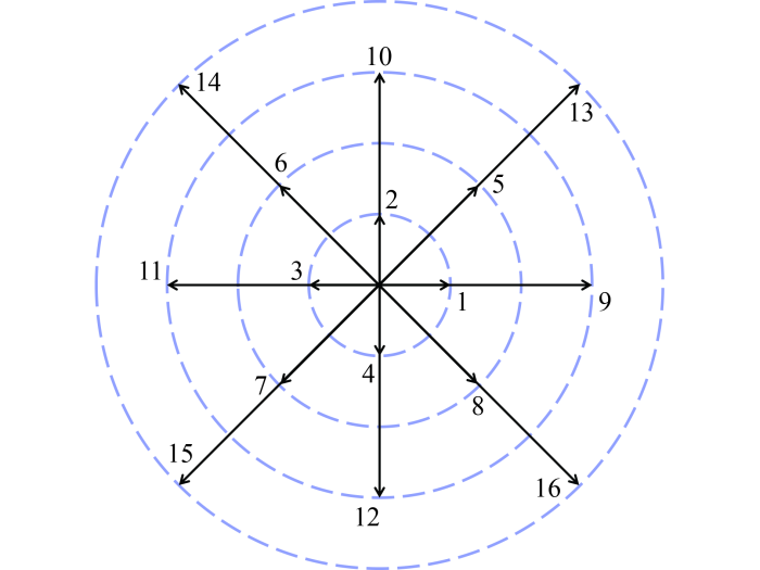
The sketch of D2V16 is shown in Fig.1. Moreover, the parameter {\eta }_i is used to describe the rotational and/or vibrational internal energies of the fluid system. {\eta }_i={\eta }_0 when i=5, 6, 7, 8, otherwise {\eta }_i=0.

Fig.1 Sketch of D2V16 discrete velocity model.

Full size|PPT slide

Via the Chapman−Enskog analysis, it is demonstrated that the compressible Navier−Stokes (NS) equations can be recovered from Eq. (1) in the continuum limit, see Eqs. (19)−(21). To this end, {f_i}^{eq} should satisfy the following matrix equation

(3)\begin{array}{r}{\hat{\mathit{f}}}^{eq}=\mathit{C}\cdot {\mathit{f}}^{eq},\end{array}

where {\hat{\mathit{f}}}^{eq} \equiv [{\widehat{f_k}}^{eq} ], {\mathit{f}}^{eq}\equiv [ {f_i}^{eq}], \mathit{C}\equiv [c_{ki} ]; {\widehat{f_k}}^{eq} is the k-th kinetic moment of {\mathit{f}}^{eq}; c_{ki} is the element of the matrix \mathit{C}, which is determined by the discrete velocity {\mathit{v}}_i and the parameter {\eta }_i. Then, the discrete equilibrium distribution function {f_i}^{eq} can be calculated as

(4)\begin{array}{r}{\mathit{f}}^{eq}={\mathit{C}}^{-1}\cdot {\hat{\mathit{f}}}^{eq},\end{array}

when the matrix \mathit{C} is invertible.

In fact, Eq. (3) is equivalent to the seven moment relations in Eqs. (22)−(28). The first three moments in Eqs. (22)−(24) describe conservative moments of mass, momentum and energy, respectively. In the three equations, the discrete equilibrium distribution function {f_i}^{eq} can be replaced by the discrete distribution function f_i. However, for the last four kinetic moments, there may be deviations when f_i replaces {f_i}^{eq}. Actually, these deviations can be used to describe the TNE effects. Consequently, the nonequilibrium manifestations are defined as below:

(5)\begin{array}{r}{\mathbf{\Delta }}_{m,n}={\mathit{M}}_{m,n}(f_i)-{\mathit{M}}_{m,n}(f_i^{eq}),\end{array}

where “ m, n” represents that the m-order tensor is reduced to the n-order tensor. In a similar way, another set of nonequilibrium manifestations are introduced as well:

(6)\begin{array}{r}{\mathbf{\Delta }}_{m,n}^{\ast }={\mathit{M}}_{m,n}^{\ast }(f_i)-{\mathit{M}}_{m,n}^{\ast }(f_i^{eq}),\end{array}

where {\mathit{v}}_i^{\ast }={\mathit{v}}_i- \mathit{u}. The difference between {\mathit{M}}_{m,n} ( {\mathbf{\Delta }}_{m,n}) and {\mathit{M}}_{m,n}^{\ast } ( {\mathbf{\Delta }}_{m,n}^{\ast }) is that {\mathit{M}}_{m,n} ( {\mathbf{\Delta }}_{m,n}) contains the macroscopic velocity \mathit{u} and the information about the thermal motion of micro particles, while {\mathit{M}}_{m,n}^{\ast } ( {\mathbf{\Delta }}_{m,n}^{\ast }) only describes the thermal motion of micro particles. Note that those definitions have specific physical meanings. {\mathbf{\Delta }}_2^{\ast } denotes the non-organized momentum flux and is related to viscosity, {\mathbf{\Delta }}_{3,1}^{\ast }, {\mathbf{\Delta }}_3^{\ast } represent the non-organized energy flux and are related to heat flux, and {\mathbf{\Delta }}_{4,2}^{\ast } stands for the flux of non-organized energy flux.

In order to depict the global TNE of the fluid system at length, several types of TNE quantities are defined here:

(7)\begin{array}{r}\mid {\mathbf{\Delta }}_2^{\ast }\mid =\sqrt{\mid {\mathrm{\Delta }}_{2xx}^{\ast }{\mid }^2+\mid {\mathrm{\Delta }}_{2xy}^{\ast }{\mid }^2+\mid {\mathrm{\Delta }}_{2yy}^{\ast }{\mid }^2},\end{array}

(8)\begin{array}{r}\mid {\mathbf{\Delta }}_{3,1}^{\ast }\mid =\sqrt{\mid {\mathrm{\Delta }}_{3,1x}^{\ast }{\mid }^2+\mid {\mathrm{\Delta }}_{3,1y}^{\ast }{\mid }^2},\end{array}

(9)\begin{array}{r}\mid {\mathbf{\Delta }}_3^{\ast }\mid =\sqrt{\mid {\mathrm{\Delta }}_{3xxx}^{\ast }{\mid }^2+\mid {\mathrm{\Delta }}_{3xxy}^{\ast }{\mid }^2+\mid {\mathrm{\Delta }}_{3xyy}^{\ast }{\mid }^2+\mid {\mathrm{\Delta }}_{3yyy}^{\ast }{\mid }^2},\end{array}

(10)\begin{array}{r}\mid {\mathbf{\Delta }}_{4,2}^{\ast }\mid =\sqrt{\mid {\mathrm{\Delta }}_{4,2xx}^{\ast }{\mid }^2+\mid {\mathrm{\Delta }}_{4,2xy}^{\ast }{\mid }^2+\mid {\mathrm{\Delta }}_{4,2yy}^{\ast }{\mid }^2}\mathtt{.}\end{array}

The total TNE quantity is given via above definitions, which characterizes the extent of deviation from the system equilibrium state:

(11)\begin{array}{r}\mid {\mathbf{\Delta }}^{\ast }\mid =\sqrt{\mid {\mathbf{\Delta }}_2^{\ast }{\mid }^2+\mid {\mathbf{\Delta }}_{3,1}^{\ast }{\mid }^2+\mid {\mathbf{\Delta }}_3^{\ast }{\mid }^2+\mid {\mathbf{\Delta }}_{4,2}^{\ast }{\mid }^2}\mathtt{.}\end{array}

The following kinds of the global average TNE strength are obtained by averaging the sum of TNE strength:

(12)\begin{array}{r}\overline{D}={\displaystyle \frac{1}{L_x{L}_y}}{\int }_0^{L_x}{\int }_0^{L_y}\mid {\mathbf{\Delta }}^{\ast }\mid \mathrm{d}x\mathrm{d}y=\frac{1}{N_x\times N_y}\sum _{i,j}\mid {\mathbf{\Delta }}^{\ast }\mid ,\end{array}

(13)\begin{array}{r}{\overline{D}}_2={\displaystyle \frac{1}{L_x{L}_y}}{\int }_0^{L_x}{\int }_0^{L_y}\mid {\mathbf{\Delta }}_2^{\ast }\mid \mathrm{d}x\mathrm{d}y=\frac{1}{N_x\times N_y}\sum _{i,j}\mid {\mathbf{\Delta }}_2^{\ast }\mid ,\end{array}

(14)\begin{array}{rl}{\overline{D}}_{3,1}& ={\displaystyle \frac{1}{L_x{L}_y}}{\int }_0^{L_x}{\int }_0^{L_y}\mid {\mathbf{\Delta }}_{3,1}^{\ast }\mid \mathrm{d}x\mathrm{d}y\\ & =\frac{1}{N_x\times N_y}\sum _{i,j}\mid {\mathbf{\Delta }}_{3,1}^{\ast }\mid ,\end{array}

where, i=1,2,\cdots , N_x, j=1,2,\cdots ,N_y, N_x=L_x/\mathrm{\Delta }x, N_y= L_y/\mathrm{\Delta }y, L_x and L_y signify the boundary length, \mathrm{\Delta } x and \mathrm{\Delta }y mean the space step.

3 Validation

In this section, three typical cases, i.e., the sound wave, thermal Couette flow and Sod shock tube, are utilized to verify the DBM.

3.1 Sound Wave

Firstly, let us prove that the sound wave can be captured by this model. To this end, the following initial configuration is considered. In a uniform field with density \rho =1.0 and velocity \mathit{u}=0.0, a small perturbation is initially imposed on the location x_0=0.2 to facilitate the propagation of the sound wave. The grid is N_x\times N_y=2000\times 1, the space step \mathrm{\Delta }x =\mathrm{\Delta }y =1.0\times {10}^{-3}, the time step \mathrm{\Delta } t=1.0\times {10}^{-4}, the relaxation time \tau =7.0\times {10}^{-5}. In addition, the outflow (periodic) boundary conditions are employed in the x ( y) direction.

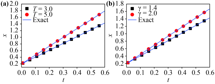
Fig.2(a) displays the position of the sound wave over time, under two different temperatures T=3.0 and 5.0, and a fixed specific heat ratio \gamma =1.4. Fig.2(b) shows the position of the sound wave, with a fixed temperature T=3.0, and two different specific heat ratios \gamma = 1.4 and 2.0. It is clear in Fig.2(a) and (b) that all simulation results coincide with the theoretical results x=x_0 +v_{s}t where the sound speed is v_s=\sqrt{\gamma T}. Therefore, the DBM can capture the sound wave well under various temperatures and specific heat ratios.

Fig.2 The position of the sound wave versus time: (a) under different temperatures; (b) under different specific heat ratios. The symbols represent the simulation results, and the solid lines denote theoretical solutions.

Full size|PPT slide

3.2 Thermal Couette flow

In this subsection, the thermal Couette flow is simulated to demonstrate that the DBM is suitable for compressible flows with flexible specific heat ratios. The physical field is between two infinite parallel plates. The distance between the two plates is H=0.4. Initially, the density is \rho =1.0, the flow velocity is \mathit{u}=0.0, and the temperature is T=1.0. The upper plate, with a fixed temperature T=1.0, moves at a constant speed of u_0=0.8. The lower plate keeps still with a fixed temperature T=1.0. The simulation grid is N_x\times N_y=1\times 200, the space step \mathrm{\Delta }x =\mathrm{\Delta }y =2.0\times {10}^{-3}, the time step \mathrm{\Delta } t=1.0\times {10}^{-5}, and the relaxation time \tau =1.0\times {10}^{-3}. Moreover, the periodic boundary conditions are applied in the x direction, and the nonequilibrium extrapolation method is adopted in the y direction.

When the thermal system reaches the stead state, there is theoretical solutions of the temperature in the y direction as follows,

(15)\begin{array}{r}T=T_0+\frac{u_0^2}{2c_p}\frac{y}{H}\left(1-\frac{y}{H}\right),\end{array}

with c_p=\gamma /(\gamma -1). The theoretical solution of the horizontal velocity reads

(16)\begin{array}{r}{u}_x=\frac{y}{H}{u}_0+\frac{2}{\pi }{u}_0\sum _{j=1}^{\mathrm{\infty }}\left[\frac{(-1{)}^j}{j}\exp \left(-j^2{\pi }^2\frac{\mu t}{\rho H^2}\right)\mathrm{s}\mathrm{i}\mathrm{n}\left(\frac{j\pi y}{H}\right)\right],\end{array}

where \mu =\tau \rho T represents the dynamic viscosity.

Fig.3 plots profiles of the temperatures and horizontal velocities in the thermal Couette flow. Fig.3(a) shows the temperatures with \gamma = 7/ 5, 9/7, and 11 /9, respectively. Fig.3(b) displays the horizontal velocities, with \gamma =7/5, at time instances t=0.0, 1.0, 4.0, 8.0, 20.0, and 60.0, respectively. The symbols denote the DBM results, and the solid lines represent theoretical solutions. It is clear that the numerical results agree well with the analytic solutions. Consequently, the DBM could describe the thermal flows with the effects of viscous shear.

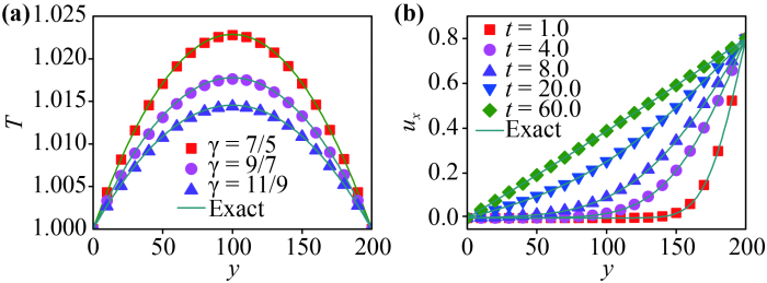
Fig.3 (a) Temperature profiles of the thermal Couette flow. The squares, circles, and triangles represent simulation results with \gamma =7 /5, 9/7, and 11 /9, respectively. (b) Horizontal velocity profiles of the thermal Couette flow with \gamma =7/5. The squares, circles, upper triangles, lower triangles and diamonds denote simulation results at time instants t=0.0, 1.0, 4.0, 8.0, 20.0, and 60.0, respectively. The solid lines represent theoretical solutions.

Full size|PPT slide

3.3 Sod shock tube

Then the Sod shock tube problem is simulated in this part. The initial configuration is

(17)\begin{array}{r}\{\begin{array}{rlr}& (\rho ,T,u,v){|}_L=(1.0,1.0,0.0,0.0),& x\le 0,\\ & (\rho ,T,u,v){|}_R=(0.125,0.8,0.0,0.0),& x>0\mathtt{.}\end{array}\end{array}

Here, the subscripts “ L” and “ R” represent the left and right sides of the initial discontinuity, respectively. The grid mesh is N_x\times N_y=2000\times 1, the space step \mathrm{\Delta }x = \mathrm{\Delta }y =1.0\times {10}^{-3}, the time step \mathrm{\Delta } t=1.0\times {10}^{-5}, the relaxation time \tau =1.0\times {10}^{-5}. The supersonic inflow (periodic) boundary conditions are applied in the x ( y) direction.

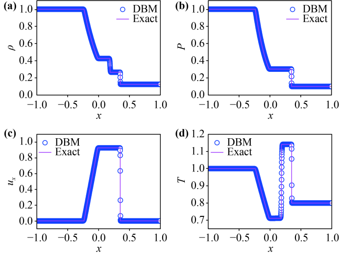
Fig.4(a)−(d) delineate profiles of the density, pressure, horizontal velocity and temperature in the Sod shock tube at a time instant t=0.2. The symbols denote the simulation results of the DBM. The solid lines are for the Riemann analytic solutions. It can be found that there are three interfaces in the evolution of the Sod shock tube. The leftmost interface is a rarefaction wavefront that covers a wide space; The middle interface separates two media with different densities and temperatures; The rightmost interface is a shock wavefront where the physical gradients are sharp. Obviously, there is nice agreement between the simulation results and Riemann analytic solutions. It is confirmed that the DBM could capture the rarefaction wave, material interface, and shock wave simultaneously.

Fig.4 Profiles of (a) the density, (b) pressure, (c) horizontal velocity and (d) temperature in the Sod shock tube. The symbols indicate the DBM results, and the solid lines stand for the Riemann solutions.

Full size|PPT slide

4 Numerical simulations

As shown in Fig.5, the initial configuration of the compressible KH instability takes the form:

Fig.5 The initial configuration of the compressible KH instability.

Full size|PPT slide

(18)\begin{array}{r}\{\begin{array}{rl}& \rho (y)=\frac{{\rho }_L+{\rho }_U}{2}-\frac{{\rho }_L-{\rho }_U}{2}\tanh (\frac{y-0.5L_y}{D_{\rho }}),\\ & u_x(y)=\frac{u_L+u_U}{2}-\frac{u_L-u_U}{2}\tanh (\frac{y-0.5L_y}{D_u}),\\ & P=P_{{}_L}=P_{{}_U},\end{array}\end{array}

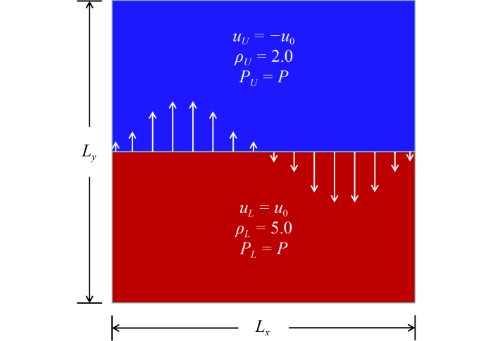
where {\rho }_U =2.0 ( {\rho }_L=5.0) is the fluid density on the upper (lower) side of the interface, u_U=-u_0 ( u_L=u_0) the tangential velocity in the upper (lower) fluid, D_u=0.008 ( D_{\rho }=0.008) the width of velocity (density) transition layer, \tanh the hyperbolic tangent function that smoothes the interface. The simulation area is L_x\times L_y=0.2\times 0.2, the space step \mathrm{\Delta }x =\mathrm{\Delta }y =2.0\times {10}^{-5}, the time step \mathrm{\Delta } t=1.0\times {10}^{-5}, the pressure P=2.5, the relaxation time \tau =4.0\times {10}^{-5}, the specific heat ratio \gamma =7 /5. An initial velocity perturbation is imposed in the y direction: u_y=A_0\sin (k x)\exp (-k\mid y-0.5L_y\mid ), where A_0=0.02 denotes the perturbation amplitude, k=2\pi / L_x the wave number. Moreover, the periodic (outflow) boundary conditions are adopted in the x ( y) direction. The grid convergence test is firstly performed to obtain the reliable simulations in Appendix B.

4.1 Hydrodynamic nonequilibrium effects

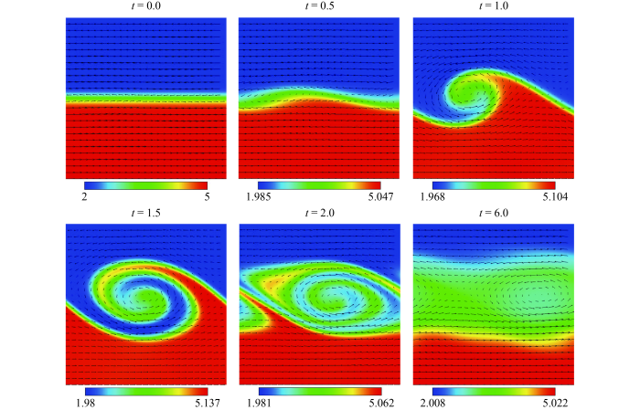
To better understand the evolution of the KH system intuitively, Fig.6 illustrates the density and velocity fields at six different time instants, with the tangential velocity u_0=0.25. Obviously, the perturbed interface begins to distort, and the transition layer widens and bends significantly at t=0.5, due to the diffusion, dissipation and viscous shear. Subsequently, at t=1.0, the system continues to develop, and a small vortex structure becomes apparent near the interface. At t=1.5, a larger regular KH vortex is observed. Afterwards, a more complex vortex appears at t=2.0. At the later stage, the mixing of the upper and lower fluids deepens, the vortex structure gradually disappears. These findings are consistent with previous studies [19,43].

Fig.6 Density and velocity fields in the case of u_0=0.25 at times t=0.0, 0.5, 1.0, 1.5, 2.0, and 6.0, respectively.

Full size|PPT slide

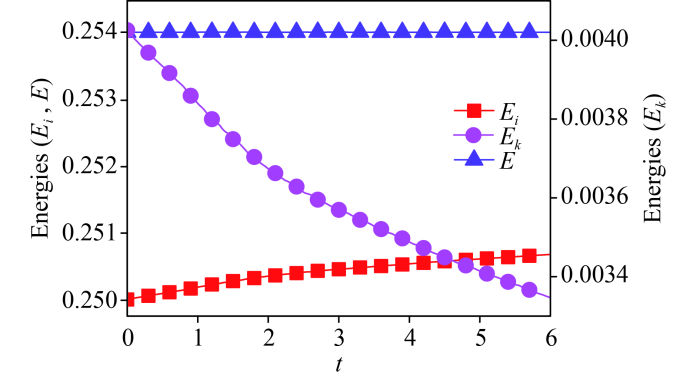
Moreover, the energy budget is an important issue in the evolution of the KH instability [56-59]. In theory, the kinetic energy is converted into the internal energy due to the effect of viscous shear as the interface morphology becomes more and more complicated. Here, the energies of the KH instability are studied. Let us introduce the following definitions: the whole internal energy \iint E_i\mathrm{d}x\mathrm{d}y=\iint \frac{1}{2} (D+n )\rho T\mathrm{d}x\mathrm{d}y, the whole kinetic energy \iint E_k\mathrm{d}x \mathrm{d}y=\iint \frac{1}{2} \rho u^2\mathrm{d}x\mathrm{d}y, and the total energy \iint E\mathrm{d}x \mathrm{d}y=\iint E_i \mathrm{d}x\mathrm{d}y+\iint E_k \mathrm{d}x\mathrm{d}y, where the integral conducted over the whole computational region. In Fig.7, the lines with squares, circles and upper triangles indicate the internal, kinetic and total energies, respectively. It can be found that the internal energy \iint E_i\mathrm{d}x\mathrm{d}y increases gradually, the kinetic energy \iint E_k\mathrm{d}x \mathrm{d}y decreases simultaneously, and the total energy \iint E\mathrm{d}x \mathrm{d}y has slight changes. That is to say, the kinetic energy changes into the internal energy in the KH process.

Fig.7 Evolution of the whole energies in the KH process. The lines with squares, circles and upper triangles are for the internal, kinetic and total energies, respectively.

Full size|PPT slide

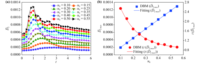
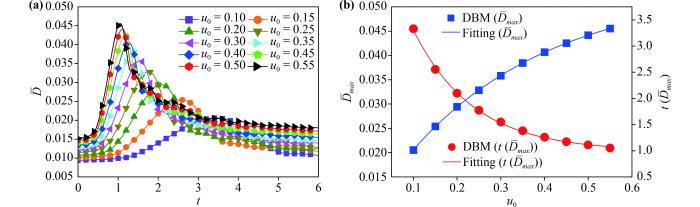
In order to study the hydrodynamic nonequilibrium effects of the compressible KH instability, ten groups of the tangential velocity u_0 are selected, where u_0 ranges from 0.10 to 0.55, with an interval of 0.05. Fig.8(a) shows the evolution of the global average density gradient in the x direction | \overline{{\mathrm{\nabla }}_x\rho } | with different values of u_0, where |\overline{{\mathrm{\nabla }}_x\rho }|={\int }_0^{L_x}{\int }_0^{L_y}|{\mathrm{\nabla }}_x\rho |\mathrm{d}x\mathrm{d}y/(L_x{L}_y). It can be seen that |\overline{{\mathrm{\nabla }}_x\rho }| increases with the growing of u_0 before the leftmost peak (of u_0=0.55) at about t=1.0. Moreover, for each u_0, | \overline{{\mathrm{\nabla }}_x\rho } | increases and then decreases as time goes on. Taking u_0=0.25 as an example, |\overline{{\mathrm{\nabla }}_x\rho }| firstly increases before t=1.7, and then decreases. Physically, there are two competitive mechanisms in the evolution of the KH instability. On the one hand, under the influence of the shear velocity, the perturbation amplitude increases in the y direction, the fluid interface is distorted and gradually elongated, which enhances the physical gradients. On the other hand, due to the dissipation and/or diffusion effects, the transition layer becomes wider and small fluid structures disappear, which suppresses the physical gradients. In the rising (descending) stage, the former (latter) mechanism plays a leading role.

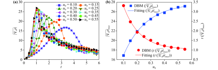
Fig.8 (a) Evolution of the global average density gradient in the x direction | \overline{{\mathrm{\nabla }}_x\rho } | under different tangential velocities u_0. (b) The relationship among |\overline{{\mathrm{\nabla }}_x\rho }{|}_{max} (defined as the maximum of | \overline{{\mathrm{\nabla }}_x\rho } |), t(| \overline{{\mathrm{\nabla }}_x\rho } {|}_{max}) (defined as the time corresponding to the peak of | \overline{{\mathrm{\nabla }}_x\rho } |) and u_0, where the symbols indicate the DBM results, the blue solid line |\overline{{\mathrm{\nabla }}_x\rho }{|}_{max}=- 19.78\exp (-5.94u_0)+ 27.87, and the red solid line t(|\overline{{\mathrm{\nabla }}_x\rho }{|}_{max})=5.26\exp ( -8.43u_0)+1.03.

Full size|PPT slide

In Fig.8(b), | \overline{{\mathrm{\nabla }}_x\rho } {|}_{max} (defined as the maximum of |\overline{{\mathrm{\nabla }}_x\rho }|), t(| \overline{{\mathrm{\nabla }}_x\rho } {|}_{max}) (defined as the time corresponding to the peak of | \overline{{\mathrm{\nabla }}_x\rho } |), and u_0 show the following relationships: |\overline{{\mathrm{\nabla }}_x\rho }{|}_{max}=-19.78 \exp (-5.94u_0)+27.87, and t(| \overline{{\mathrm{\nabla }}_x\rho } {|}_{max})= 5.26\exp (-8.43u_0) +1.03. Obviously, | \overline{{\mathrm{\nabla }}_x\rho } {|}_{max} increases exponentially while t(| \overline{{\mathrm{\nabla }}_x\rho } {|}_{max}) decreases exponentially, with the increasing of u_0. Furthermore, it can be found that |\overline{{\mathrm{\nabla }}_x\rho }{|}_{max} is also a function of t(| \overline{{\mathrm{\nabla }}_x\rho } {|}_{max}), namely, |\overline{{\mathrm{\nabla }}_x\rho }{|}_{max}=27.01 \exp (-0.35t(|\overline{{\mathrm{\nabla }}_x\rho } {|}_{max}))+8.39, and | \overline{{\mathrm{\nabla }}_x\rho } {|}_{max} declines exponentially as t(| \overline{{\mathrm{\nabla }}_x\rho } {|}_{max}) increases. In fact, for a larger u_0, the system evolves rapidly, it takes less time to reach the peak value, the density structure in the x direction is more complex, and |\overline{{\mathrm{\nabla }}_x\rho }{|}_{max} becomes larger [20,25,26].

Fig.9(a) plots the evolution of the global average density gradient in the y direction |\overline{{\mathrm{\nabla }}_y\rho }| under different tangential velocities u_0, where | \overline{{\mathrm{\nabla }}_y\rho } | ={\int }_0^{L_x}{\int }_0^{L_y}|{\mathrm{\nabla }}_y\rho |\mathrm{d}x\mathrm{d}y/(L_x{L}_y). The global average density gradient in the y direction |\overline{{\mathrm{\nabla }}_y\rho }| keeps constant initially, then increases, and decreases afterwards. And |\overline{{\mathrm{\nabla }}_y\rho }| grows with the increase of u_0 before the leftmost peak. Taking u_0=0.25 as an example, it can be found that |\overline{{\mathrm{\nabla }}_y\rho }| almost keeps constant from t=0.0 to t=0.5. At the beginning, the upper and lower density near the system interface is quite different. And the interface twists slightly, the density declines monotonously along the y direction, hence |\overline{{\mathrm{\nabla }}_y\rho }| is almost constant. Then, from t=0.5 to t=1.8, |\overline{{\mathrm{\nabla }}_y\rho }| increases rapidly and forms a peak around t=1.8. In this process, the fluid interface is extended vertically, a regular vortex forms gradually, and the density no longer changes monotonously in the y direction. In addition, compared with Fig.5, it can be found that | \overline{{\mathrm{\nabla }}_y\rho } | increases rapidly when a vortex structure emerges. Finally, the physical gradients become smooth, the fluid interface gets blurred, and the vortex gradually disappears, as the fluid mixing deepens.

Fig.9 (a) Evolution of the global average density gradient in the y direction | \overline{{\mathrm{\nabla }}_y\rho } | under different tangential velocities u_0. (b) The relationship among |\overline{{\mathrm{\nabla }}_y\rho }{|}_{max}, t(| \overline{{\mathrm{\nabla }}_y\rho } {|}_{max}) and u_0, where the symbols indicate the DBM results, the blue solid line |\overline{{\mathrm{\nabla }}_y\rho }{|}_{max}=- 42.67\exp (-4.34u_0)+ 58.49, and the red solid line t(|\overline{{\mathrm{\nabla }}_y\rho }{|}_{max})=5.61\exp ( -8.26u_0)+1.08.

Full size|PPT slide

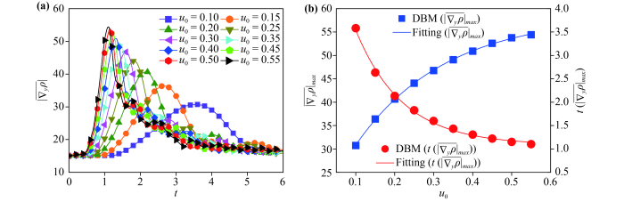
Furthermore, the relationships among |\overline{{\mathrm{\nabla }}_y\rho }{|}_{max}, t(| \overline{{\mathrm{\nabla }}_y\rho } {|}_{max}) and u_0 are shown in Fig.9 (b). Specifically, |\overline{{\mathrm{\nabla }}_y\rho }{|}_{max}=- 42.67\exp (-4.34u_0)+ 58.49, and t(|\overline{{\mathrm{\nabla }}_y\rho } {|}_{max})= 5.61\exp (-8.26u_0) +1.08. | \overline{{\mathrm{\nabla }}_y\rho } {|}_{max} ascents exponentially and t(| \overline{{\mathrm{\nabla }}_y\rho } {|}_{max}) descents exponentially as u_0 becomes large. Additionally, the formula | \overline{{\mathrm{\nabla }}_y\rho } {|}_{max}=58.59\exp (- 0.56t(| \overline{{\mathrm{\nabla }}_y\rho } {|}_{max}))+22.93 can also be obtained. Clearly, the larger t(|\overline{{\mathrm{\nabla }}_y\rho } {|}_{max}), the smaller |\overline{{\mathrm{\nabla }}_y\rho }{|}_{max}, in an exponential declining trend. Physically, the larger u_0 is, the faster the system develops, the more complex the density changes, the larger the peak value becomes, and the less time it takes to reach the peak value.

Fig.10(a) delineates the evolution of the global average density gradient | \overline{\mathrm{\nabla }\rho }| under different u_0 values, where |\overline{\mathrm{\nabla }\rho } | ={\int }_0^{L_x}{\int }_0^{L_y}|\mathrm{\nabla } \rho |dxdy/(L_x{L}_y). In fact, the tendency of |\overline{\mathrm{\nabla }\rho } | can be obtained from the analysis of | \overline{{\mathrm{\nabla }}_x\rho } | and |\overline{{\mathrm{\nabla }}_y\rho }| in Fig.8(a) and Fig.8(a). Similarly, Fig.10(b) shows the relationship among |\overline{\mathrm{\nabla }\rho }{|}_{max}, t(| \overline{\mathrm{\nabla }\rho }{|}_{max}) and u_0. It can be seen that |\overline{\mathrm{\nabla }\rho } {|}_{max}=-48.35\exp (-4.55u_0)+68.03 and t(|\overline{\mathrm{\nabla }\rho }{|}_{max})=5.27\exp ( -7.94u_0)+1.05. With the increase of u_0, |\overline{\mathrm{\nabla }\rho } {|}_{max} increases by an exponential function, while t(| \overline{\mathrm{\nabla }\rho }{|}_{max}) decreases exponentially. Besides, |\overline{\mathrm{\nabla }\rho } | declines exponentially as t(|\overline{\mathrm{\nabla }\rho } {|}_{max}) grows, i.e., |\overline{\mathrm{\nabla }\rho } {|}_{max}=65.96\exp (- 0.52t(| \overline{\mathrm{\nabla }\rho }{|}_{max}))+26.36. The physical mechanisms are similar to those in Fig.8(b) and Fig.9(b).

Fig.10 (a) Evolution of the global average density gradient |\overline{\mathrm{\nabla }\rho } | under different tangential velocities u_0. (b) The relationship among |\overline{\mathrm{\nabla }\rho }{|}_{max}, t(| \overline{\mathrm{\nabla }\rho }{|}_{max}) and u_0, where the symbols indicate the DBM results, the blue solid line | \overline{\mathrm{\nabla }\rho }{|}_{max}=-48.35 \exp (- 4.55u_0)+68.03, and the red solid line t(| \overline{\mathrm{\nabla }\rho }{|}_{max})=5.27\exp ( -7.94u_0)+1.05.

Full size|PPT slide

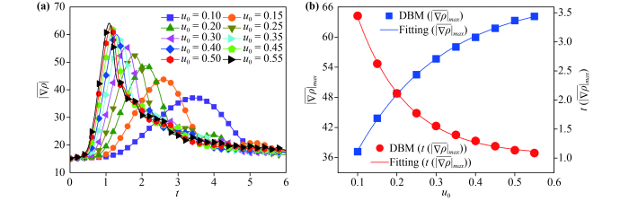
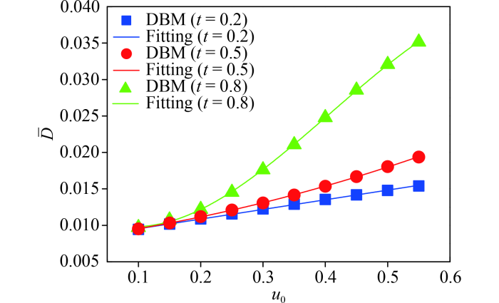
Fig.11(a) shows the simulation results and fitting curves of |\overline{\mathrm{\nabla }\rho }| at three different times, with various tangential velocities u_0. At the time t=0.1, the relation between |\overline{\mathrm{\nabla }\rho }| and u_0 reads | \overline{\mathrm{\nabla }\rho }|(t=0.1 )=15.29+0.12u_0 +0.56u_0^2. It can be found that |\overline{\mathrm{\nabla }\rho } | increases slightly with the increasing of u_0 at the early stage. For different values of u_0, the systems evolve slowly, and the interface has few changes initially. At a later time t=0.5, the relation is |\overline{\mathrm{\nabla }\rho } | (t=0.5 )=16.13-8.93u_0+25.50u_0^2. Clearly, the differences between |\overline{\mathrm{\nabla }\rho } | become apparent. Physically, with the action of the shear, the fluid interface with a larger u_0 has twisted earlier, while the one with smaller u_0 has no obvious change. At t=0.8, it can be found that |\overline{\mathrm{\nabla }\rho } | (t=0.8 )=(0.23-1.12u_0+4.66 u_0^2-3.59u_0^3)\times {10}^2. For the system with a larger u_0, a vortex forms distinctly and the density changes with a strongly nonlinear trend. However, for a smaller u_0, the fluid interface starts to curl or still has no significant change.

Fig.11 (a) The simulation results and fitting functions of |\overline{\mathrm{\nabla }\rho } | with various tangential velocities u_0 at three different times: |\overline{\mathrm{\nabla }\rho } | (t=0.1 )=15.29+0.12u_0 +0.56u_0^2, |\overline{\mathrm{\nabla }\rho }|( t=0.5)=16.13-8.93u_0+ 25.50u_0^2, and |\overline{\mathrm{\nabla }\rho } | (t=0.8 )=(0.23-1.12u_0+4.66 u_0^2-3.59u_0^3)\times {10}^2. (b) The relationship between t(|\overline{\mathrm{\nabla }\rho } | ) (the time corresponding to |\overline{\mathrm{\nabla }\rho } |) and u_0 at three different values: t(| \overline{\mathrm{\nabla }\rho }|=20)= 2.60\exp (-7.96u_0)+ 0.51, t(| \overline{\mathrm{\nabla }\rho }|=25)= 3.65\exp (-8.94u_0)+ 0.61, and t(|\overline{\mathrm{\nabla }\rho } | =35)=6.34\exp (-10.71u_0) +0.77.

Full size|PPT slide

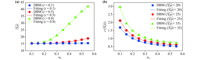
Fig.11(b) displays the relation between t(| \overline{\mathrm{\nabla }\rho }|) (the time corresponding to | \overline{\mathrm{\nabla }\rho }|) and tangential velocity u_0 at three different values. From the formula t(|\overline{\mathrm{\nabla }\rho }|=20 )= 2.60 \exp (-7.96u_0)+0.51, it can be found that the larger u_0, the smaller t(|\overline{\mathrm{\nabla }\rho } | =20). Via the formulae t(| \overline{\mathrm{\nabla }\rho }|= 25)=3.65\exp (-8.94u_0) +0.61 and t(|\overline{\mathrm{\nabla }\rho }|=35 )=6.34\exp (- 10.71u_0)+0.77, the development trend of t(| \overline{\mathrm{\nabla }\rho }|=25) and t(|\overline{\mathrm{\nabla }\rho }|=35 ) is similar to that of t(| \overline{\mathrm{\nabla }\rho }|=20). It indicates that the larger u_0 becomes, the more rapidly the system evolves, and the less time for |\overline{\mathrm{\nabla }\rho } | to reach the same value takes. Moreover, the interface structure has complicated, and |\overline{\mathrm{\nabla }\rho } | is large as time goes on.

4.2 Thermodynamic nonequilibrium effects

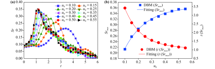
Next, the TNE behaviors in the KH instability are discussed and analyzed. Fig.12(a) illustrates the global average viscous stress tensor strength {\overline{D}}_2 versus time. In general, {\overline{D}}_2 rises first and then declines over time, and increases with the increasing of u_0. Particularly, taking u_0=0.25 as an example, {\overline{D}}_2 increases slowly from t=0.0 to 0.5. During this stage, as the viscous shear takes effect, the fluid interface gradually curls up. Then, from t=0.5 to 1.5, {\overline{D}}_2 grows rapidly, the peak is observed around t=1.5 and a regular vortex emerges. When t>1.5, on account of the dissipation and/or diffusion, the KH vortex vanishes gradually and {\overline{D}}_2 declines. Fig.12(b) shows the relationship of {\overline{D}}_{2max}, t({\overline{D}}_{2max}) and u_0. The specific expressions are {\overline{D}}_{2max}=( -0.04+2.45 u_0)\times {10}^{-3} and t({\overline{D}}_{2max}) =3.41\exp (-6.87u_0) +0.85. {\overline{D}}_{2max} increases linearly and t({\overline{D}}_{2max}) decreases exponentially as u_0 increases [60,61]. Furthermore, it is easy to obtain the formula {\overline{D}}_{2max}=[7.45\exp (-2.13t({\overline{D}}_{2max}) )+0.21 ]\times {10}^{-3}. That is, {\overline{D}}_2 decreases exponentially with the increasing of t({\overline{D}}_{2max}). Physically, the larger u_0 is, the stronger the shear force is, and the faster two fluids mix.

Fig.12 (a) Evolution of the global average viscous stress tensor strength {\overline{D}}_2 under different tangential velocities u_0. (b) The relationship among {\overline{D}}_{2max}, t({\overline{D}}_{2max}) and u_0, where the symbols indicate the DBM results, the blue solid line {\overline{D}}_{2max}=( -0.04+2.45 u_0)\times {10}^{-3}, and the red solid line t({\overline{D}}_{2max})=3.41 \exp (-6.87u_0)+0.85.

Full size|PPT slide

To understand the relationship between u_0 and {\overline{D}}_2 in the early stage, Fig.13 plots the relations between {\overline{D}}_2 and u_0 at three various times t=0.2, 0.5, and 0.8, respectively. Details are as follows: {\overline{D}}_2(t=0.2 )=(0.02+1.00 u_0)\times {10}^{-3}, {\overline{D}}_2(t=0.5)= (0.01+0.93u_0+ 1.02u_0^2)\times {10}^{-3}, and {\overline{D}}_2(t=0.8 )=(0.09-0.42u_0+9.09 u_0^2-8.17u_0^3)\times {10}^{-3}. Specifically, the larger u_0 is, the greater the viscous shear becomes, the faster the system evolves, the earlier the vortex forms, and the larger {\overline{D}}_2 is. Additionally, in the initial stage, the system evolves almost linearly with the increasing of u_0. And the system evolves nonlinearly afterwards, hence there is a nonlinear relation between {\overline{D}}_2 and u_0 as time goes on.

Fig.13 The simulation results and fitting functions of the global average viscous stress tensor strength {\overline{D}}_2 with various tangential velocities u_0 at three different times: {\overline{D}}_2(t=0.2)= (0.02+1.00u_0 )\times {10}^{-3}, {\overline{D}}_2(t=0.5)= (0.01+0.93u_0+ 1.02u_0^2)\times {10}^{-3}, and {\overline{D}}_2(t=0.8 )=(0.09-0.42u_0+9.09 u_0^2-8.17u_0^3)\times {10}^{-3}.

Full size|PPT slide

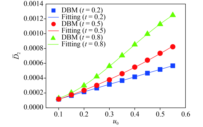
Fig.14 describes the evolution of the TNE quantities {\overline{D}}_{3,1x}, {\overline{D}}_{3,1y} and {\overline{D}}_{3,1}. From Fig.14(a), for any u_0, {\overline{D}}_{3,1x} rises first then declines over time. Furthermore, before the leftmost peak, {\overline{D}}_{3,1x} increases with the growing of u_0. At the beginning, there is little temperature change in the x direction, hence the corresponding temperature gradients are almost zero, and {\overline{D}}_{3,1x} develops from zero. Afterwards, due to the viscous shear, the interface is elongated and twists gradually and the temperature field in the x direction starts to get complicated. Therefore, {\overline{D}}_{3,1x} rises rapidly. In the later stage, although the contact area of two fluids increases continuously, the vortex and small structures are dissipated gradually due to the diffusion and heat conduction, and consequently {\overline{D}}_{3,1x} reduces.

Fig.14 Evolution of the global average heat flux strength: (a) in the x direction {\overline{D}}_{3,1x}, (b) in the y direction {\overline{D}}_{3,1y} and (c) {\overline{D}}_{3,1}, with different tangential velocities u_0. (d) The relationship among {\overline{D}}_{3,1max}, t({\overline{D}}_{3,1max} ) and u_0, where the symbols indicate the DBM results, the blue solid line {\overline{D}}_{3,1max}= [-0.82 \exp (-5.05u_0)+1.10 ]\times {10}^{-2}, and the red solid line t({\overline{D}}_{3,1max})= 5.30\exp (-8.03u_0) +1.05.

Full size|PPT slide

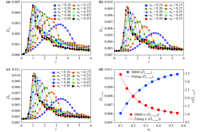
Fig.14(b) illustrates the evolution of {\overline{D}}_{3,1y}. Similar to {\overline{D}}_{3,1x} in Fig.14(a), there is a peak of {\overline{D}}_{3,1y} in each case. For all cases, {\overline{D}}_{3,1y} keeps constant in the early stage (roughly before t=0.5), then increases, and decreases later. And {\overline{D}}_{3,1y} increases with the increasing of u_0 roughly before the leftmost peak. In fact, in the initial phase, there is a temperature difference between the two fluids, hence there is heat conduction across the interface and the value of {\overline{D}}_{3,1y} is nonzero. Meanwhile, the temperature varies monotonously in the y direction, so {\overline{D}}_{3,1y} keeps constant. Then, the fluid structure becomes more and more complicated, the physical field in the y direction changes no longer monotonously, and the heat exchange is enhanced, hence {\overline{D}}_{3,1y} increases obviously. In the later stage, the interface gets blurred, the physical gradients become smooth, and {\overline{D}}_{3,1y} decreases.

From Fig.14(c), it can be found that the evolutionary trend of {\overline{D}}_{3,1} is similar to that of {\overline{D}}_{3,1y}. That is because the physical mechanism of {\overline{D}}_{3,1} can be acquired from that of {\overline{D}}_{3,1x} and {\overline{D}}_{3,1y} and dominated by the second component. Through the fitting method, the relationship among {\overline{D}}_{3,1max}, t({\overline{D}}_{3,1max}) and u_0 can be expressed as {\overline{D}}_{3,1max}=[-0.82\exp (-5.05u_0) +1.10]\times {10}^{-2} and t({\overline{D}}_{3,1max})=5.30\exp (-8.03u_0) +1.05, as seen in Fig.14(d). Furthermore, the formula {\overline{D}}_{3,1max}=[1.10\exp (-0.45t({\overline{D}}_{3,1max})) +0.37]\times {10}^{-2} can be derived as well. Physically, the fluid mixing deepens, the temperature gradients and the heat exchange are enhanced, in the system with a large u_0. Additionally, the rapid evolution of the system and the large fluid contact area are caused by the large u_0.

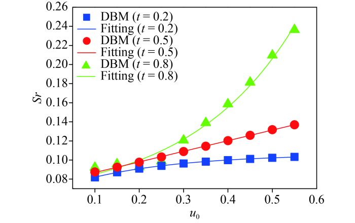
Fig.15(a) plots the relationships between {\overline{D}}_{3,1} and u_0 at three time instants t=0.1, 0.5, and 0.8, respectively. Physically, as the fluid system evolves from t=0.1 to 0.8, the temperature field becomes more complex, and {\overline{D}}_{3,1} increases. Especially, the fitting functions are {\overline{D}}_{3,1}(t=0.1 )=(26.40-0.09u_0+0.44 u_0^2)\times {10}^{-4}, {\overline{D}}_{3,1}(t=0.5)=( 2.70-0.63 u_0+1.73 u_0^2)\times {10}^{-3}, and {\overline{D}}_{3,1}(t=0.8 )=(0.04-1.59u_0+6.29 u_0^2-4.61u_0^3)\times {10}^{-2}, respectively. In addition, at an early time t=0.1, {\overline{D}}_{3,1} increases slightly with the growing of u_0. In the later period t=0.8, the influence of u_0 is obvious.

Fig.15 (a) The simulation results and fitting functions of the global average heat flux strength {\overline{D}}_{3,1} with various tangential velocities u_0 at three different times: {\overline{D}}_{3,1}(t=0.1)=( 26.40-0.09u_0+0.44 u_0^2)\times {10}^{-4}, {\overline{D}}_{3,1}(t=0.5)=( 2.70-0.63u_0+1.73 u_0^2)\times {10}^{-3}, and {\overline{D}}_{3,1}(t=0.8 )=(0.04-1.59u_0+6.29 u_0^2-4.61u_0^3)\times {10}^{-2}. (b) The relationship between t({\overline{D}}_{3,1}) and u_0 at three different values: t({\overline{D}}_{3,1}=0.0035)=3.02\exp (-8.78u_0)+0.59, t({\overline{D}}_{3,1}=0.0045)= 4.33\exp (-9.70u_0)+ 0.70, and t({\overline{D}}_{3,1}=0.0055)=5.84\exp (-10.53u_0)+ 0.78.

Full size|PPT slide

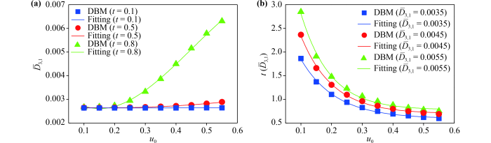
Fig.15(b) shows the relation between the velocity u_0 and the time t({\overline{D}}_{3,1}) when {\overline{D}}_{3,1} reaches a given value. Here three different cases {\overline{D}}_{3,1}=35, 45, and 55 are under consideration. The following fitting formulae t({\overline{D}}_{3,1}= 0.0035 )=3.02\exp (- 8.78u_0)+0.59, t({\overline{D}}_{3,1}=0.0045)= 4.33\exp (-9.70u_0) +0.70, and t({\overline{D}}_{3,1}=0.0055)= 5.84\exp (-10.53u_0)+ 0.78 can be obtained. It is obvious that t({\overline{D}}_{3,1}=0.0035) declines exponentially when u_0 increases in each case. The tendencies of t({\overline{D}}_{3,1}=0.0045), t({\overline{D}}_{3,1}=0.0055) and t({\overline{D}}_{3,1}=0.0035) are similar to each other. The larger {\overline{D}}_{3,1} is, the more thoroughly the upper and lower fluids mix, and the more time it takes. In addition, the larger u_0 is, the more significantly the temperature gradients increase, the faster the heat exchange becomes, and the less time it requires to reach the same value.

To have a deeper understanding of nonequilibrium effects in the KH instability, the global average TNE strength \overline{D} is discussed next. As plotted in Fig.16(a), \overline{D} ascents first and descents later, and increases with the increasing of u_0 before the leftmost peak. Physically, there are two competitive physical mechanisms that affect the TNE effects during the KH process. On the one hand, the material interface between the two fluids is elongated and widened as the fluid structures become complicated, which promotes the development of the nonequilibrium region. On the one hand, in the evolution of the KH instability, the physical gradients are smoothed by the dissipation and/or diffusion, which weakens the local TNE strength. In the early stage, the former physical mechanism plays a major role, which leads to the rapid increase of \overline{D}. On the contrary, in the later period, \overline{D} gradually decreases due to the decrease of the local TNE effect. Fig.16(b) presents the relationship among {\overline{D}}_{max}, t({\overline{D}}_{max}) and u_0, as expressed in formulae {\overline{D}}_{max}=[-4.53\exp (- 3.06u_0)+5.40]\times {10}^{-2} and t({\overline{D}}_{max})=4.81\exp (-7.30u_0) +0.99. And the formula {\overline{D}}_{max}=[6.52\exp (-0.74 t({\overline{D}}_{max}))+1.52] \times {10}^{-2} is obtained by combining above two formulae. {\overline{D}}_{max} declines exponentially as t({\overline{D}}_{max}) increases. In fact, for a large u_0, the viscous shear is promoted, the macroscopic physical gradients are enhanced, and the nonequilibrium region increases. Therefore, {\overline{D}}_{max} increases and t({\overline{D}}_{max}) decreases when u_0 increases.

Fig.16 (a) Evolution of the global average TNE strength \overline{D} under different tangential velocities u_0. (b) The relationship among {\overline{D}}_{max}, t({\overline{D}}_{max}) and u_0, where the symbols indicate the DBM results, the blue solid line {\overline{D}}_{max}=[-4.53\exp (- 3.06u_0)+ 5.40 ]\times {10}^{-2}, and the red solid line t({\overline{D}}_{max})=4.81\exp (-7.30u_0)+0.99.

Full size|PPT slide

The relationship between \overline{D} and u_0 at three different times are shown in Fig.17. Obviously, \overline{D} and u_0 are linear, quadratic, and cubic functions for t=0.2, 0.5 and 0.8, respectively. To be specific, the relationships are as follows: \overline{D}(t=0.2 )=(0.83+1.32u_0)\times {10}^{-2}, \overline{D}(t=0.5 )=(0.83+1.12 u_0+1.66 u_0^2)\times {10}^{-2}, and \overline{D}( t=0.8)=(0.12 -0.51u_0+3.07u_0^2-2.51 u_0^3)\times {10}^{-1}. Physically, at the three times, the larger u_0 becomes, the more complicated the fluid interface changes, the larger the nonequilibrium area becomes, the more rapidly the physical gradients increase, and hence the stronger the TNE grows.

Fig.17 The simulation results and fitting functions of the global average TNE strength \overline{D} with various tangential velocities u_0 at three different times: \overline{D}(t= 0.2)=(0.83+ 1.32 u_0)\times {10}^{-2}, \overline{D}(t= 0.5)=(0.83+1.12 u_0+1.66 u_0^2)\times {10}^{-2}, and \overline{D}( t=0.8)=(0.12 -0.51u_0+3.07u_0^2-2.51 u_0^3)\times {10}^{-1}.

Full size|PPT slide

To further analyze the evolution of the global TNE, the proportion of the nonequilibrium region Sr is introduced [38], where Sr is equal to the ratio of the nonequilibrium area to the total area of the physical system. The nonequilibrium area is where the nonequilibrium intensity is greater than a given threshold. In the simulation, the Sr is carried out at the threshold 0.06. To have an intuitive understanding, the contours of the nonequilibrium region in the evolution of the KH instability are shown in Fig.18. It can be found that, at an early time instant t=0.02, the nonequilibrium strength near the interface is relatively large, because the physical gradients between two fluids are quite sharp and the local TNE effects are directly associated with the physical gradients. As the system evolves (for example, at a time instant t=0.5), the interface between the two fluids is extended vertically, and the transition layer widens gradually. Later (from t=1.0 to t=2.0), the interface twists significantly, and a vortex and small structures emerge. Finally ( t>6.0), as two fluids mix sufficiently, the vortex and small structures are dissipated, and the physical gradients get smooth gradually.

Fig.18 Contours of the nonequilibrium strength in the case of u_0=0.25 at times t=0.02, 0.5, 1.0, 1.5, 2.0, and 6.0, respectively.

Full size|PPT slide

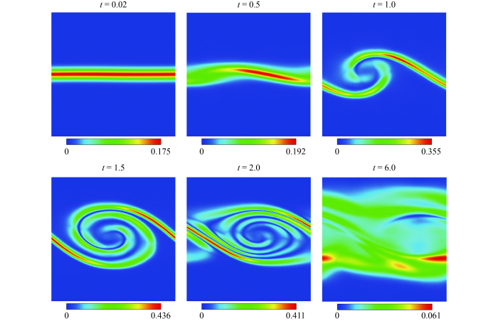
Fig.19(a) illustrates the proportion of the nonequilibrium region Sr versus the time t. Similarly, ten cases are under consideration with different tangential velocities u_0. It is clear that the nonequilibrium region increases and then decreases with time, and it increases with the growing of u_0 before the leftmost peak. Physically, on the one hand, as the fluid interface is elongated in the KH process, the nonequilibrium region increases simultaneously. Meanwhile, due to the dissipation and/or diffusion effects, the interface is widened and the nonequilibrium region becomes wide. On the other hand, because the local physical gradients decrease, the nonequilibrium effects weaken. When the nonequilibrium intensity is less than the given threshold, this point does not belong to the nonequilibrium area any longer. The former two physical mechanisms promote the increasing of Sr, while the latter leads to the decreasing of Sr.

Fig.19 (a) Evolution of the proportion of the nonequilibrium region Sr under different tangential velocities u_0. (b) The relationship among S{r}_{max}, t(S{r}_{max}) and u_0, where the symbols indicate the DBM results, the blue solid line S r_{max}=[-2.76\exp (- 6.07u_0)+3.66]\times {10}^{-1}, and the red solid line t(S{r}_{max})=5.18\exp ( -8.09u_0)+1.08.

Full size|PPT slide

In addition, as displayed in Fig.19(b), the relationship among S{r}_{max}, t(S{r}_{max}) and u_0 are S r_{max}=[-2.76\exp (- 6.07u_0)+3.66]\times {10}^{-1} and t(S{r}_{max})=5.18\exp ( -8.09u_0)+ 1.08, respectively. It can be found that the formula S r_{max}=0.42-0.06t(S{r}_{max}) is derived, and S{r}_{max} decreases linearly with the increasing of t(S{r}_{max}). In fact, the larger u_0 is, the deeper and faster two fluids mix, the greater the nonequilibrium strength becomes. Consequently, the larger S{r}_{max}, and the smaller t(S{r}_{max}).

Fig.20 describes the relationship between Sr and u_0 at three different times. The fitting formulae are Sr(t=0.2 )=[-0.38\exp (-4.54u_0)+1.06]\times {10}^{-1}, Sr(t=0.5 )=(0.76+1.11u_0)\times {10}^{-1}, and Sr(t= 0.8)=[3.43\exp(- 3.17u_0)+3.56]\times {10}^{-2}, respectively. It can be found that the relationship between Sr and u_0 are negative exponential, linear and positive exponential at the time instants t=0.2, 0.5, and 0.8, respectively. To be specific, Sr changes little with the increasing of u_0 at the time t=0.2. At this moment, the system evolution is in the initial stage and the nonequilibrium strength is relatively weak in each case. As time goes by, u_0 has a significant effect on the fluid system, and hence the differences of Sr are large as well.

Fig.20 The simulation results and fitting functions of the proportion of the nonequilibrium region Sr with various tangential velocities u_0 at three different times: Sr(t=0.2 )= [-0.38\exp (- 4.54u_0)+1.06]\times {10}^{-1}, Sr(t=0.5)=( 0.76+1.11u_0)\times {10}^{-1}, and Sr(t= 0.8)=[3.43\exp (-3.17 u_0)+3.56] \times {10}^{-2}.

Full size|PPT slide

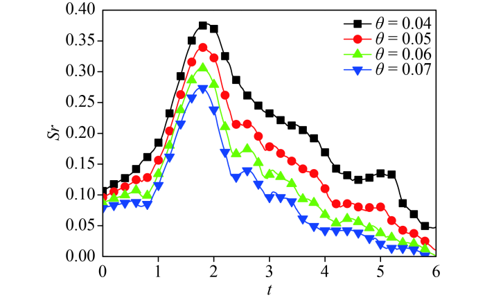
To have a better understanding of the TNE effects in the evolution of the KH instability, Fig.21 depicts the proportion of the nonequilibrium region versus the time with various thresholds of the TNE strength \theta =0.04, 0.05, 0.06, and 0.07, respectively. The tangential velocity is chosen as u_0=0.25. Clearly, the simulation results in Fig.21 are in line with those in Fig.18. For all cases, the nonequilibrium areas increase firstly and decrease afterwards, and hence there is a high peak. With the increasing of the threshold, the TNE region declines.

Fig.21 The proportion of the nonequilibrium region Sr versus the time t, with four different threshold values \theta in the case of u_0=0.25. The black line, red line, green line, and blue line correspond to threshold values \theta =0.04, 0.05, 0.06, and 0.07, respectively.

Full size|PPT slide

5 Conclusions

In this paper, the impacts of the tangential velocity on the hydrodynamic and thermodynamic nonequilibrium effects are investigated during the compressible KH process by using the DBM. Ten cases with different tangential velocities are simulated and analyzed in detail. Firstly, the global average density gradients |\overline{\mathrm{\nabla }\rho }|, | \overline{{\mathrm{\nabla }}_x\rho } |, and |\overline{{\mathrm{\nabla }}_y\rho }| are discussed. On the whole, | \overline{\mathrm{\nabla }\rho }| and |\overline{{\mathrm{\nabla }}_x\rho }| increase and then decrease with time, and | \overline{{\mathrm{\nabla }}_y\rho } | keeps constant firstly, then increases, and decreases later. All these density gradients increase as the tangential velocity increases in the early period. With the increasing of the tangential velocity, the system evolves more rapidly and becomes more complicated. Physically, there are two competitive mechanisms in the KH process. On the one hand, under the influence of the shear velocity, the perturbation amplitude increases, the fluid interface is distorted and gradually elongated, which enhances the physical gradients. On the other hand, due to the dissipation and/or diffusion effects, the transition layer becomes wider and small fluid structures disappear, which suppresses the physical gradients. In the early (later) stage, the former (latter) mechanism plays a leading role.

Next, the detailed TNE effects are measured and analyzed in the KH process. (i) The global average viscous stress tensor strength {\overline{D}}_2 firstly increases and then decreases, and it becomes stronger for a larger tangential velocity u_0. The maximum of {\overline{D}}_2 is a linear function of u_0, which is consistent with the theory^[60,^61]. (ii) The global average heat flux strength {\overline{D}}_{3,1} and {\overline{D}}_{3,1x} increase and then decrease with time, and {\overline{D}}_{3,1y} keeps constant firstly, then increases, and decreases afterwards. All global average heat fluxes increase with the increasing of the tangential velocity in the early period. On the one hand, the local heat exchange reduces when the physical gradients decrease. On the other hand, the whole area of heat flux increases as the contact interface becomes large. (iii) The global average TNE strength \overline{D} firstly increases and decreases afterwards, and it increases with the increasing tangential velocity u_0 in the early period. Physically, the decreasing physical gradients weaken the TNE strength, while the increasing of nonequilibrium region enhances the TNE intensity. (iv) The proportion of the nonequilibrium region Sr increases firstly and then declines, and it is larger for a higher u_0 in the early stage. Physically, the nonequilibrium region increases as the fluid interface is elongated due to the viscous shear and is widened by the dissipation and/or diffusion. Meanwhile, the TNE effects weaken because the local physical gradients decrease. The former two physical mechanisms promote the increasing of Sr, while the latter leads to the decreasing of Sr. These results enrich our perception in the compressible KH instability, and provide another perspective for further exploration of physical mechanisms in fluid dynamics.

6 Appendix A

The recovered compressible NS equations take the following form:

(19)\begin{array}{r}\frac{\mathrm{\partial }\rho }{\mathrm{\partial }t}+\mathrm{\nabla }\cdot (\rho \mathit{u})=0,\end{array}

(20)\begin{array}{r}\frac{\mathrm{\partial }}{\mathrm{\partial }t}(\rho \mathit{u})+\mathrm{\nabla }\cdot (\rho \mathit{u}\mathit{u}+p\mathit{I}+\mathit{P})=0,\end{array}

(21)\begin{array}{r}\frac{\mathrm{\partial }}{\mathrm{\partial }t}[\rho (e+\frac{|\mathit{u}{|}^2}{2})]+\mathrm{\nabla }\cdot [\rho \mathit{u}(e+T+\frac{|\mathit{u}{|}^2}{2})+\mathit{J}+\mathit{P}\cdot \mathit{u}]=0,\end{array}

where e=(D+n)T/2 the internal energy per unit mass, D the space dimension, n the number of extra degrees of freedom other than translational freedom, \kappa =(D+ n+ 2)\mu /2 the coefficient of thermal conductivity, \mathit{P}= -\mu [\mathrm{\nabla } \mathit{u}+(\mathrm{\nabla }\mathit{u}{)}^{\mathrm{T}}-\frac{2}{D+n}( \mathrm{\nabla }\cdot \mathit{u})\mathit{I}] the viscous stress, \mathit{J}= -\kappa \mathrm{\nabla }T the heat flux.

Seven kinetic moment formulae about f_i^{eq} are:

(22)\begin{array}{r}{M}_0^{eq}:\sum _i{f}_i^{eq}=\rho ,\end{array}

(23)\begin{array}{r}{M}_1^{eq}:\sum _i{f}_i^{eq}{\mathit{v}}_i=\rho \mathit{u},\end{array}

(24)\begin{array}{r}{M}_{2,0}^{eq}:\sum _i{f}_i^{eq}({\mathit{v}}_i\cdot {\mathit{v}}_i+{{\eta }_i}^2)=\rho [(D+n)T+\mathit{u}\cdot \mathit{u}],\end{array}

(25)\begin{array}{r}{M}_2^{eq}:\sum _i{f}_i^{eq}{\mathit{v}}_i{\mathit{v}}_i=\rho (T\mathit{I}+\mathit{u}\cdot \mathit{u}),\end{array}

(26)\begin{array}{rl}{M}_{3,1}^{eq}:\sum _i{f}_i^{eq}({\mathit{v}}_i\cdot {\mathit{v}}_i+{{\eta }_i}^2){\mathit{v}}_i=& \rho \mathit{u}[(D+n+2)T\\ & +\mathit{u}\cdot \mathit{u}],\end{array}

(27)\begin{array}{rl}{M}_3^{eq}:\sum _i{f}_i^{eq}{\mathit{v}}_i{\mathit{v}}_i{\mathit{v}}_i=& \rho [T({\mathit{u}}_{\alpha }{\mathbf{e}}_{\beta }{\mathbf{e}}_{\chi }{\delta }_{\beta \chi }+{\mathit{u}}_{\beta }{\mathbf{e}}_{\alpha }{\mathbf{e}}_{\chi }{\delta }_{\alpha \chi }\\ & +{\mathit{u}}_{\chi }{\mathbf{e}}_{\alpha }{\mathbf{e}}_{\beta }{\delta }_{\alpha \beta })+\mathit{u}\mathit{u}\mathit{u}],\end{array}

(28)\begin{array}{r}{M}_{4,2}^{eq}:\sum _i{f}_i^{eq}({\mathit{v}}_i\cdot {\mathit{v}}_i+{{\eta }_i}^2){\mathit{v}}_i{\mathit{v}}_i=\rho T[(D+n+2)T+\mathit{u}\cdot \mathit{u}]\\ {\mathit{e}}_{\alpha }{\mathit{e}}_{\beta }{\delta }_{\alpha \beta }+\rho \mathit{u}\mathit{u}[(D+n+4)T+\mathit{u}\cdot \mathit{u}],\end{array}

where {\mathit{e}}_{\alpha } represents the unit vector in the \alpha direction, {\delta }_{\alpha \beta } the Kronecker function, \alpha, \beta, \chi = x or y.

7 Appendix B

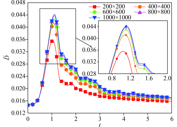
In this section, a grid convergence test is performed to establish an optimal grid. displays the profiles of \overline{D} in the KH process under five different grids N_x\times N_y=200\times 200, 400\times 400, 600\times 600, 800\times 800, and 1000\times 1000, respectively. The time step is \mathrm{\Delta } t=1.0\times {10}^{-5}, the relaxation time \tau =4.0\times {10}^{-5}, the specific heat ratio \gamma =7 /5. As shown in the legend, the lines with different symbols represent the simulation results in the five cases. It is found that, for each case, the global TNE strength increases firstly and then decreases. And the numerical differences between the adjacent cases reduce with the increasing of mesh grid. That is to say, numerical errors become smaller for a high resolution. To be specific, the results of grids 800\times 800 and 1000\times 1000 are quite close to each other. Considering the numerical error and resolution, the grid N_x\times N_y=1000\times 1000 is chosen, namely the space step \mathrm{\Delta } x(=\mathrm{\Delta }y)=2.0\times {10}^{-5}, in this paper.

Fig. B1 Grid convergence test of simulations of the KH instability: the global average TNE intensity \overline{D} versus the time t, with five different mesh grids. The lines with squares, circles, diamonds, upper and lower triangles correspond to mesh grids N_x\times N_y=200\times 200, 400 \times 400, 600 \times 600, 800 \times 800, and 1000 \times 1000, respectively.

Full size|PPT slide

Acknowledgements

This work was supported by the National Natural Science Foundation of China (Grant Nos. 51806116 and 11875001) and the Natural Science Foundation of Fujian Provinces (Grant Nos. 2021J01652 and 2021J01655).

References

1 S.Chandrasekhar, Hydrodynamic and Hydromagnetic Stability, Oxford University Press, London, 1961

2 C.K. Batchelor, An Introduction to Fluid Dynamics, Cambridge University Press, Cambridge, 2000

3 H.Luce, L.Kantha, M.Yabuki, H.Hashiguchi. Atmospheric Kelvin−Helmholtz billows captured by the MU radar, lidars and a fish-eye camera. Earth Planets Space , 2018, 70( 1): 162

4 L.F. Wang, W.H. Ye, X.T. He, J.F. Wu, Z.F. Fan, C.Xue, H.Y. Guo, W.Y. Miao, Y.T. Yuan, J.Q. Dong, G.Jia, J.Zhang, Y.J. Li, J.Liu, M.Wang, Y.K. Ding, W.Y. Zhang. Theoretical and simulation research of hydrodynamic instabilities in inertial-confinement fusion implosions. Sci. China: Phys. Mech. Astron. , 2017, 60( 5): 055201

5 R.V. Coelho, M.Mendoza, M.M. Doria, H.J. Herrmann. Kelvin−Helmholtz instability of the Dirac fluid of charge carriers on graphene. Phys. Rev. B , 2017, 96( 18): 184307

6 V.V. Mishin, V.M. Tomozov. Kelvin−Helmholtz instability in the solar atmosphere, solar wind and geomagnetosphere. Sol. Phys. , 2016, 291( 11): 3165

7 A.Petrarolo, M.Kobald, S.Schlechtriem. Understanding Kelvin−Helmholtz instability in paraffin-based hybrid rocket fuels. Exp. Fluids , 2018, 59( 4): 62

8 R.K. Azadboni, A.Heidari, J.X. Wen. Numerical studies of flame acceleration and onset of detonation in homogenous and inhomogeneous mixture. J. Loss Prev. Process Ind. , 2020, 64 : 104063

9 X.Y. Zhang, S.P. Li, B.Y. Yang, N.F. Wang. Flow structures of over-expanded supersonic gaseous jets for deep-water propulsion. Ocean Eng. , 2020, 213 : 107611

10 X.F. Xiao, G.B. Zhao, W.X. Zhou, S.Martynenko. Large-eddy simulation of transpiration cooling in turbulent channel with porous wall. Appl. Therm. Eng. , 2018, 145 : 618

11 W.Huang, Z.Du, L.Yan, Z.Xia. Supersonic mixing in airbreathing propulsion systems for hypersonic flights. Prog. Aerosp. Sci. , 2019, 109 : 100545

12 E.C. Harding, J.F. Hansen, O.A. Hurricane, R.P. Drake, H.F. Robey, C.C. Kuranz, B.A. Remington, M.J. Bono, M.J. Grosskopf, R.S. Gillespie. Observation of a Kelvin−Helmholtz instability in a high-energydensity plasma on the omega laser. Phys. Rev. Lett. , 2009, 103( 4): 045005

13 M.K. Awasthi, R.Asthana, G.Agrawal. Viscous correction for the viscous potential flow analysis of Kelvin−Helmholtz instability of cylindrical flow with heat and mass transfer. Int. J. Heat Mass Transf. , 2014, 78 : 251

14 B.Akula, P.Suchandra, M.Mikhaeil, D.Ranjan. Dynamics of unstably stratified free shear flows: An experimental investigation of coupled Kelvin−Helmholtz and Rayleigh−Taylor instability. J. Fluid Mech. , 2017, 816 : 619

15 C.D. Lin, A.G. Xu, G.C. Zhang, Y.J. Li, S.Succi. Polarcoordinate lattice Boltzmann modeling of compressible flows. Phys. Rev. E , 2014, 89( 1): 013307

16 A.G. Xu, G.C. Zhang, Y.B. Gan, F.Chen, X.J. Yu. Lattice Boltzmann modeling and simulation of compressible flows. Front. Phys. , 2012, 7( 5): 582

17 J.P. Parker, C.P. Caulfield, R.R. Kerswell. The effects of Prandtl number on the nonlinear dynamics of Kelvin−Helmholtz instability in two dimensions. J. Fluid Mech. , 2021, 915 : A37

18 V.Mohan, A.Sameen, B.Srinivasan, S.S. Girimaji. Influence of Knudsen and Mach numbers on Kelvin−Helmholtz instability. Phys. Rev. E , 2021, 103( 5): 053104

19 Y.B. Gan, A.G. Xu, G.C. Zhang, C.D. Lin, H.L. Lai, Z.P. Liu. Nonequilibrium and morphological characterizations of Kelvin−Helmholtz instability in compressible flows. Front. Phys. , 2019, 14( 4): 43602

20 H.G. Lee, J.Kim. Two-dimensional Kelvin− Helmholtz instabilities of multi-component fluids. Eur. J. Mech. BFluids , 2015, 49 : 77

21 K.S. Kim, M.H. Kim. Simulation of the Kelvin−Helmholtz instability using a multi-liquid moving particle semi-implicit method. Ocean Eng. , 2017, 130 : 531

22 M.J. Yao, W.Q. Shang, Y.Zhang, H.Gao, D.X. Zhang, P.Y. Liu. Numerical analysis of Kelvin−Helmholtz instability in inclined walls. Chin. J. Comput. Phys. , 2019, 36 : 403

23 K.I. Ebihara, T.Watanabe. Lattice Boltzmann simulation of the interfacial growth of the horizontal stratified two-phase flow. Int. J. Mod. Phys. B , 2003, 17( 01n02): 113

24 Y.B. Gan, A.G. Xu, G.C. Zhang, Y.J. Li. Lattice Boltzmann study on Kelvin−Helmholtz instability: Roles of velocity and density gradients. Phys. Rev. E , 2011, 83( 5): 056704

25 Y.G. Li, X.G. Geng, Z.J. Liu, H.P. Wang, D.Y. Zang. Simulating Kelvin−Helmholtz instability using dissipative particle dynamics. Fluid Dyn. Res. , 2018, 50( 4): 045512

26 W.Q. Shang, Y.Zhang, Z.Q. Chen, Z.P. Yuan, B.H. Dong. Numerical simulation of two-dimensional Kelvin−Helmholtz instabilities using a front tracking method. Chin. J. Comput. Mech. , 2018, 35 : 424

27 G.A. Hoshoudy, M.K. Awasthi. Compressibility effects on the Kelvin−Helmholtz and Rayleigh−Taylor instabilities between two immiscible fluids flowing through a porous medium. Eur. Phys. J. Plus , 2020, 135( 2): 169

28 E.P. Budiana. The meshless numerical simulation of Kelvin−Helmholtz instability during the wave growth of liquid−liquid slug flow. Comput. Math. Appl. , 2020, 80( 7): 1810

29 R.M. McMullen, M.C. Krygier, J.R. Torczynski, M.A. Gallis. Navier−Stokes equations do not describe the smallest scales of turbulence in gases. Phys. Rev. Lett. , 2022, 128( 11): 114501

30 A.G. Xu, C.D. Lin, G.C. Zhang, Y.J. Li. Multiple-relaxation-time lattice Boltzmann kinetic model for combustion. Phys. Rev. E , 2015, 91( 4): 043306

31 C.D. Lin, K.H. Luo. Discrete Boltzmann modeling of unsteady reactive flows with nonequilibrium effects. Phys. Rev. E , 2019, 99( 1): 012142

32 X.L. Su, C.D. Lin. Nonequilibrium effects of reactive flow based on gas kinetic theory. Commum. Theor. Phys. , 2022, 74( 3): 035604

33 Y.B. Gan, A.G. Xu, G.C. Zhang, S.Succi. Discrete Boltzmann modeling of multiphase flows: Hydrodynamic and thermodynamic nonequilibrium effects. Soft Matter , 2015, 11( 26): 5336

34 Y.B. Gan, A.G. Xu, G.C. Zhang, Y.D. Zhang, S.Succi. Discrete Boltzmann trans-scale modeling of high-speed compressible flows. Phys. Rev. E , 2018, 97( 5): 053312

35 H.L. Lai, A.G. Xu, G.C. Zhang, Y.B. Gan, Y.J. Li, S.Succi. Nonequilibrium thermohydrodynamic effects on the Rayleigh−Taylor instability in compressible flows. Phys. Rev. E , 2016, 94( 2): 023106

36 D.M. Li, H.L. Lai, A.G. Xu, G.C. Zhang, C.D. Lin, Y.B. Gan. Discrete Boltzmann simulation of Rayleigh−Taylor instability in compressible flows. Acta Physica Sinica , 2018, 67( 8): 080501

37 H.Y. Ye, H.L. Lai, D.M. Li, Y.B. Gan, C.D. Lin, L.Chen, A.G. Xu. Knudsen number effects on two-dimensional Rayleigh−Taylor instability in compressible fluid: Based on a discrete Boltzmann method. Entropy (Basel) , 2020, 22( 5): 500

38 L.Chen, H.L. Lai, C.D. Lin, D.M. Li. Specific heat ratio effects of compressible Rayleigh−Taylor instability studied by discrete Boltzmann method. Front. Phys. , 2021, 16( 5): 52500

39 L.Chen, H.L. Lai, C.D. Lin, D.M. Li. Numerical study of multimode Rayleigh−Taylor instability by using the discrete Boltzmann method. Acta Aerodyn. Sin. , 2022, 40 : 1

40 C.D. Lin, A.G. Xu, G.C. Zhang, Y.J. Li. An efficient two-dimensional discrete Boltzmann model of detonation. Adv. Condens. Matter Phys. , 2015, 4( 3): 102

41 F.Chen, A.G. Xu, G.C. Zhang. Collaboration and competition between Richtmyer−Meshkov instability and Rayleigh-Taylor instability. Phys. Fluids , 2018, 30( 10): 102105

42 Y.D. Zhang, A.G. Xu, G.C. Zhang, Z.H. Chen, P.Wang. Discrete Boltzmann method for non-equilibrium flows: Based on Shakhov model. Comput. Phys. Commun. , 2019, 238 : 50

43 C.D. Lin, K.H. Luo, Y.B. Gan, Z.P. Liu. Kinetic simulation of nonequilibrium Kelvin−Helmholtz instability. Commum. Theor. Phys. , 2019, 71( 1): 132

44 D.J. Zhang, A.G. Xu, Y.D. Zhang, Y.J. Li. Two-fluid discrete Boltzmann model for compressible flows: Based on ellipsoidal statistical Bhatnagar−Gross−Krook. Phys. Fluids , 2020, 32( 12): 126110

45 F.Chen, A.G. Xu, Y.D. Zhang, Q.K. Zeng. Morphological and nonequilibrium analysis of coupled Rayleigh−Taylor−Kelvin−Helmholtz instability. Phys. Fluids , 2020, 32( 10): 104111

46 C.D. Lin, K.H. Luo, A.G. Xu, Y.B. Gan, H.L. Lai. Multiple-relaxation-time discrete Boltzmann modeling of multicomponent mixture with nonequilibrium effects. Phys. Rev. E , 2021, 103( 1): 013305

47 F.Chen, A.G. Xu, Y.D. Zhang, Y.B. Gan, B.B. Liu, S.Wang. Effects of the initial perturbations on the Rayleigh−Taylor−Kelvin−Helmholtz instability system. Front. Phys. , 2022, 17( 3): 33505

48 R.Benzi, S.Succi, M.Vergassola. The lattice Boltzmann equation: Theory and applications. Phys. Rep. , 1992, 222( 3): 145

49 X.Y. He S. Y. Chen G.D. Doolen, A novel thermal model for the lattice Boltzmann method in incompressible limit, J. Comput. Phys . 146(1), 282 ( 1998)

50 Z.H. Chai, B.C. Shi. Multiple-relaxation-time lattice Boltzmann method for the Navier−Stokes and nonlinear convection-diffusion equations: Modeling, analysis, and elements. Phys. Rev. E , 2020, 102( 2): 023306

51 Q.Li, H.Yang, R.Z. Huang. Lattice Boltzmann simulation of solidliquid phase change with nonlinear density variation. Phys. Fluids , 2021, 33( 12): 123302

52 Z.D. Wang Y.K. Wen Y.H. Qian, A novel thermal lattice Boltzmann model with heat source and its application in incompressible flow, Appl. Math. Comput . 427, 127167 ( 2022)

53 A.G. Xu, J.Chen, J.H. Song, D.W. Chen, Z.H. Chen. Progress of discrete Boltzmann study on multiphase complex flows. Acta Aerodyn. Sin. , 2021, 39 : 138

54 A.G. Xu, J.H. Song, F.Chen, K.Xie, Y.J. Ying. Modeling and analysis methods for complex fields based on phase space. Chin. J. Comput. Phys. , 2021, 38 : 631

55 A.G. Xu, Y.M. Shan, F.Chen, Y.B. Gan, C.D. Lin. Progress of mesoscale modeling and investigation of combustion multiphase flow. Acta Aero. Astro. Sin. , 2021, 42 : 625842

56 G.P. Klaassen, W.R. Peltier. Evolution of finite amplitude Kelvin−Helmholtz billows in two spatial dimensions. J. Atmos. Sci. , 1985, 42( 12): 1321

57 G.P. Klaassen, W.R. Peltier. The effect of prandtl number on the evolution and stability of Kelvin−Helmholtz billows. Geophys. Astrophys. Fluid Dyn. , 1985, 32( 1): 23

58 R.Fatehi, M.S. Shadloo, M.T. Manzari. Numerical investigation of two-phase secondary Kelvin−Helmholtz instability. Proc. Instit. Mech. Eng. C:J. Mech. Eng. Sci. , 2014, 228( 11): 1913

59 K.Kiuchi, P.Cerdá-Durán, K.Kyutoku, Y.Sekiguchi, M.Shibata. Efficient magnetic-field amplification due to the Kelvin−Helmholtz instability in binary neutron star mergers. Phys. Rev. D , 2015, 92( 12): 124034

60 Y.D. Zhang, A.G. Xu, G.C. Zhang, C.M. Zhu, C.D. Lin. Kinetic modeling of detonation and effects of negative temperature coefficient. Combust. Flame , 2016, 173 : 483

61 C.D. Lin K.H. Luo L.L. Fei S.Succi, A multi-component discrete Boltzmann model for nonequilibrium reactive flows, Sci. Rep . 7(1), 14580 ( 2017)