PDF(639 KB)

Effective lateral dispersion of momentum, heat and mass in bubbling fluidized beds
Frontiers of Chemical Science and Engineering ›› 2024, Vol. 18 ›› Issue (12) : 151.
PDF(639 KB)
PDF(639 KB)
Effective lateral dispersion of momentum, heat and mass in bubbling fluidized beds
The lateral dispersion of bed material in a bubbling fluidized bed is a key parameter in the prediction of the effective in-bed heat transfer and transport of heterogenous reactants, properties important for the successful design and scale-up of thermal and/or chemical processes. Computational fluid dynamics simulations offer means to investigate such beds in silico and derive effective parameters for reduced-order models. In this work, we use the Eulerian-Eulerian two-fluid model with the kinetic theory of granular flow to perform numerical simulations of solids mixing and heat transfer in bubbling fluidized beds. We extract the lateral solids dispersion coefficient using four different methods: by fitting the transient response of the bed to (1) an ideal heat or (2) mass transfer problem, (3) by extracting the time-averaged heat transfer behavior and (4) through a momentum transfer approach in an analogy with single-phase turbulence. The method (2) fitting against a mass transfer problem is found to produce robust results at a reasonable computational cost when assessed against experiments. Furthermore, the gas inlet boundary condition is shown to have a significant effect on the prediction, indicating a need to account for nozzle characteristics when simulating industrial cases.

effective dispersion / heat transfer / mass transfer / mixing / gas-solid fluidized bed
Tab.1 The simulation cases evaluated in the present work |
| Case | dp/mm | u0/umf | H0/m | Lz/m | Simulation study | |
|---|---|---|---|---|---|---|
| Lx/m | Inlet boundary condition | |||||
| HiVoid-small-uniform | 0.3 | 33.7 | 0.2 | 0.6 | 0.6 | Uniform |
| HiVoid-large-uniform | 1.2 | Uniform | ||||
| LoVoid-small-uniform | 0.9 | 2.3 | 0.45 | 1.29 | 0.99 | Uniform |
| LoVoid-large-uniform | 1.995 | Uniform | ||||
| LoVoid-small-nozzle | 0.99 | Nozzles | ||||
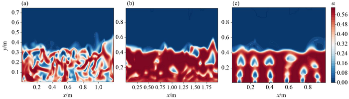
Fig.2 A visual comparison of instantaneous volume fraction fields in the different beds studied. (a) The HiVoid case with smaller sand corresponds to the solids used in the experiments of Sette et al. [33], and (b, c) the LoVoid cases with larger sand corresponds to the solids used in the experiments of Martinez Castilla et al. [37]. The LoVoid-small-nozzle case (c) employs “nozzle” inlet boundary condition instead of the uniform “porous plate” inlet boundary condition used in the other cases (a, b). |
| [1] |
YangW C. Handbook of Fluidization and Fluid-Particle Systems. Taylor & Francis, 2003
|
| [2] |
Kraussler M , Binder M , Schindler P , Hofbauer H . Hydrogen production within a polygeneration concept based on dual fluidized bed biomass steam gasification. Biomass and Bioenergy, 2018, 111: 320–329
CrossRef
ADS
Google scholar
|
| [3] |
Heinze C , May J , Peters J , Ströhle J , Epple B . Techno-economic assessment of polygeneration based on fluidized bed gasification. Fuel, 2019, 250: 285–291
CrossRef
ADS
Google scholar
|
| [4] |
Eschenbacher A , Jensen P A , Henriksen U B , Ahrenfeldt J , Jensen C D , Li C , Enemark-Rasmussen K , Duus J Ø , Mentzel U V , Jensen A D . Catalytic upgrading of tars generated in a 100 kWth low temperature circulating fluidized bed gasifier for production of liquid bio-fuels in a polygeneration scheme. Energy Conversion and Management, 2020, 207: 112538
CrossRef
ADS
Google scholar
|
| [5] |
Salman C A , Naqvi M , Thorin E , Yan J . Impact of retrofitting existing combined heat and power plant with polygeneration of biomethane: a comparative techno-economic analysis of integrating different gasifiers. Energy Conversion and Management, 2017, 152: 250–265
CrossRef
ADS
Google scholar
|
| [6] |
Salman C A , Omer C B . Process modelling and simulation of waste gasification-based flexible polygeneration facilities for power, heat and biofuels production. Energies, 2020, 13(16): 4264
CrossRef
ADS
Google scholar
|
| [7] |
Gadsbøll R Ø , Clausen L R , Thomsen T P , Ahrenfeldt J , Henriksen U B . Flexible TwoStage biomass gasifier designs for polygeneration operation. Energy, 2019, 166: 939–950
CrossRef
ADS
Google scholar
|
| [8] |
Yu P , Luo Z , Wang Q , Fang M . Life cycle assessment of transformation from a sub-critical power plant into a polygeneration plant. Energy Conversion and Management, 2019, 198: 111801
CrossRef
ADS
Google scholar
|
| [9] |
Naqvi M , Dahlquist E , Yan J , Naqvi S R , Nizami A S , Salman C A , Danish M , Farooq U , Rehan M , Khan Z .
CrossRef
ADS
Google scholar
|
| [10] |
Zhao K , Thunman H , Pallarès D , Ström H . Control of the solids retention time by multi-staging a fluidized bed reactor. Fuel Processing Technology, 2017, 167: 171–182
CrossRef
ADS
Google scholar
|
| [11] |
Salehi M S , Askarishahi M , Radl S . Quantification of solid mixing in bubbling fluidized beds via two-fluid model simulations. Industrial & Engineering Chemistry Research, 2020, 59(22): 10606–10621
CrossRef
ADS
Google scholar
|
| [12] |
Diba M F , Karim M R , Naser J . Numerical modelling of a bubbling fluidized bed combustion: a simplified approach. Fuel, 2020, 277: 118170
CrossRef
ADS
Google scholar
|
| [13] |
Jiradilok V , Gidaspow D , Breault R W . Computation of gas and solid dispersion coefficients in turbulent risers and bubbling beds. Chemical Engineering Science, 2007, 62(13): 3397–3409
CrossRef
ADS
Google scholar
|
| [14] |
Oke O , Lettieri P , Salatino P , Solimene R , Mazzei L . Numerical simulations of lateral solid mixing in gas-fluidized beds. Chemical Engineering Science, 2014, 120: 117–129
CrossRef
ADS
Google scholar
|
| [15] |
Hernández-Jiménez H , Sánchez-Prieto J , Cano-Pleite E , Soria-Verdugo A . Lateral solids meso-mixing in pseudo-2D fluidized beds by means of TFM simulations. Powder Technology, 2018, 334: 183–191
CrossRef
ADS
Google scholar
|
| [16] |
Yu M , Miller D C , Biegler L T . Dynamic reduced order models for simulating bubbling fluidized bed adsorbers. Industrial & Engineering Chemistry Research, 2015, 54(27): 6959–6974
CrossRef
ADS
Google scholar
|
| [17] |
Wang H , Li Z , Li Y , Cai N . Reduced-order model for CaO carbonation kinetics measured using micro-fluidized bed thermogravimetric analysis. Chemical Engineering Science, 2021, 229: 116039
CrossRef
ADS
Google scholar
|
| [18] |
Yuan T , Cizmas P G , O’Brien T . A reduced-order model for a bubbling fluidized bed based on proper orthogonal decomposition. Computers & Chemical Engineering, 2005, 30(2): 243–259
CrossRef
ADS
Google scholar
|
| [19] |
Li C , Dai Z , Sun Z , Wang F . Modeling of an opposed multiburner gasifier with a reduced-order model. Industrial & Engineering Chemistry Research, 2013, 52(16): 5825–5834
CrossRef
ADS
Google scholar
|
| [20] |
Saastamoinen J J . Simplified model for calculation of devolatilization in fluidized beds. Fuel, 2006, 85(17-18): 2388–2395
CrossRef
ADS
Google scholar
|
| [21] |
Kaushal P , Abedi J . A simplified model for biomass pyrolysis in a fluidized bed reactor. Journal of Industrial and Engineering Chemistry, 2010, 16(5): 748–755
CrossRef
ADS
Google scholar
|
| [22] |
Gómez-Barea A , Leckner B . Modeling of biomass gasification in fluidized bed. Progress in Energy and Combustion Science, 2010, 36(4): 444–509
CrossRef
ADS
Google scholar
|
| [23] |
Kaushal P , Tyagi R . Advanced simulation of biomass gasification in a fluidized bed reactor using ASPEN PLUS. Renewable Energy, 2017, 101: 629–636
CrossRef
ADS
Google scholar
|
| [24] |
Nikku M , Bordbar H , Myöhänen K , Hyppänen T . Effects of heterogeneous flow on carbon conversion in gas-solid circulating fluidized beds. Fuel, 2020, 280: 118623
CrossRef
ADS
Google scholar
|
| [25] |
Sternéus J , Johnsson F , Leckner B . Characteristics of gas mixing in a circulating fluidised bed. Powder Technology, 2002, 126(1): 28–41
CrossRef
ADS
Google scholar
|
| [26] |
Chirone R , Miccio F , Scala F . On the relevance of axial and transversal fuel segregation during the FB combustion of a biomass. Energy & Fuels, 2004, 18(4): 1108–1117
CrossRef
ADS
Google scholar
|
| [27] |
OkeOLettieriPSalatinoPMazzeiL. CFD simulations of lateral solid mixing in fluidized beds. CFB-11: Proceedings of the 11th International Conference on Fluidized Bed Technology, 2014, 287–292
|
| [28] |
Oke O , Lettieri P , Salatino P , Solimene R , Mazzei L . Eulerian modeling of lateral solid mixing in gas-fluidized suspensions. Procedia Engineering, 2015, 102: 1491–1499
CrossRef
ADS
Google scholar
|
| [29] |
Vandewalle L A , Francia V , Van Geem K M , Marin G B , Coppens M O . Solids lateral mixing and compartmentalization in dynamically structured gas-solid fluidized beds. Chemical Engineering Journal, 2022, 430: 133063
CrossRef
ADS
Google scholar
|
| [30] |
Luo G , Cheng L , Ma Z , Li L , Li Z , Wang P , Li L , Rong H . MP-PIC simulation on solid dispersion in a 350 MW CFB boiler. Industrial & Engineering Chemistry Research, 2022, 61(45): 16857–16868
CrossRef
ADS
Google scholar
|
| [31] |
Luo G , Cheng L , Kang Q , Zhang Q , Li K , Guo Q , Li W . Investigation on solid dispersion in a CFB dense region with bluetooth tracking method and MP-PIC simulation. Powder Technology, 2023, 429: 118892
CrossRef
ADS
Google scholar
|
| [32] |
Liu D , Chen X . Lateral solids dispersion coefficient in large-scale fluidized beds. Combustion and Flame, 2010, 157(11): 2116–2124
CrossRef
ADS
Google scholar
|
| [33] |
Sette E , Pallarès D , Johnsson F . Experimental evaluation of lateral mixing of bulk solids in a fluid-dynamically down-scaled bubbling fluidized bed. Powder Technology, 2014, 263: 74–80
CrossRef
ADS
Google scholar
|
| [34] |
Oke O , Van Wachem B , Mazzei L . Lateral solid mixing in gas-fluidized beds: CFD and DEM studies. Chemical Engineering Research & Design, 2016, 114: 148–161
CrossRef
ADS
Google scholar
|
| [35] |
BakshiA. Multiscale continuum simulations of fluidization: bubbles, mixing dynamics and reactor scaling. Dissertation of PhD degree. Boston: Massachusetts Institute of Technology, 2017
|
| [36] |
Askarishahi M , Salehi M S , Molaei Dehkordi A . Numerical investigation on the solid flow pattern in bubbling gas-solid fluidized beds: effects of particle size and time averaging. Powder Technology, 2014, 264: 466–476
CrossRef
ADS
Google scholar
|
| [37] |
Martinez Castilla G , Larsson A , Lundberg L , Johnsson F , Pallarès D . A novel experimental method for determining lateral mixing of solids in fluidized beds—quantification of the splash-zone contribution. Powder Technology, 2020, 370: 96–103
CrossRef
ADS
Google scholar
|
| [38] |
PallarèsDDíezPJohnssonF. Experimental analysis of fuel mixing patterns in a fluidized bed. The 12th International Conference on Fluidization-New Horizons in Fluidization Engineering, 2007
|
| [39] |
Norouzi H R , Mostoufi N , Mansourpour Z , Sotudeh-Gharebagh R , Chaouki J . Characterization of solids mixing patterns in bubbling fluidized beds. Chemical Engineering Research & Design, 2011, 89(6): 817–826
CrossRef
ADS
Google scholar
|
| [40] |
Olsson J , Pallarès D , Johnsson F . Lateral fuel dispersion in a large-scale bubbling fluidized bed. Chemical Engineering Science, 2012, 74: 148–159
CrossRef
ADS
Google scholar
|
| [41] |
Farzaneh M , Almstedt A E , Johnsson F , Pallarès D , Sasic S . The crucial role of frictional stress models for simulation of bubbling fluidized beds. Powder Technology, 2015, 270: 68–82
CrossRef
ADS
Google scholar
|
| [42] |
Ostermeier P , DeYoung S , Vandersickel A , Gleis S , Spliethoff H . Comprehensive investigation and comparison of TFM, DenseDPM and CFD-DEM for dense fluidized beds. Chemical Engineering Science, 2019, 196: 291–309
CrossRef
ADS
Google scholar
|


 PDF(639 KB)
补充材料
FCE-24056-OF-GG_suppl_1 (638 KB)
 Tab.1 The simulation cases evaluated in the present work
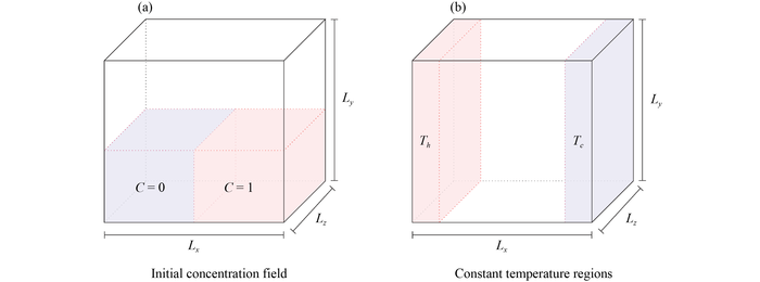
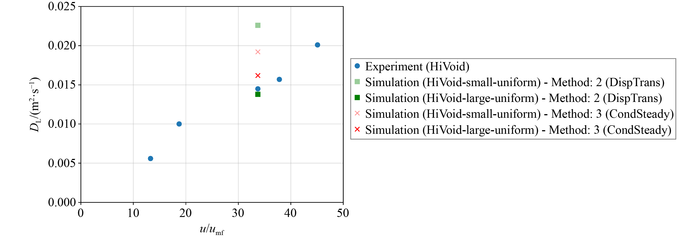
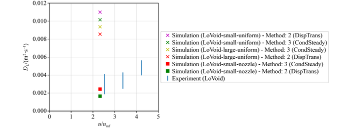
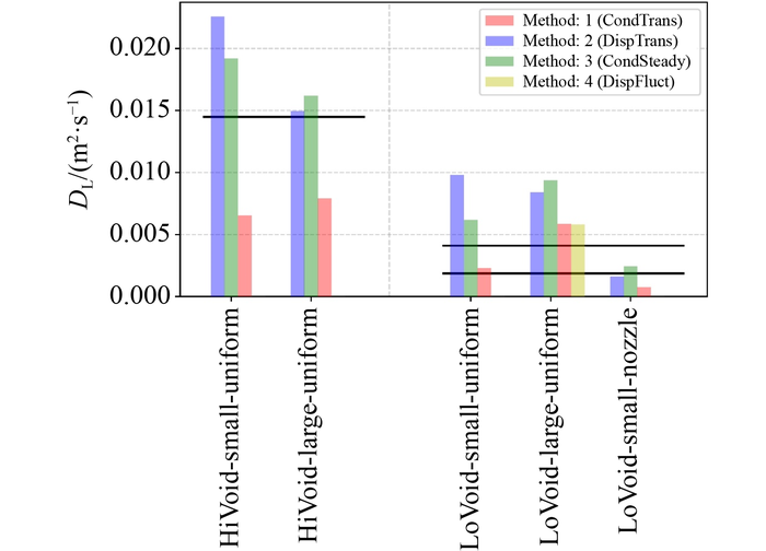
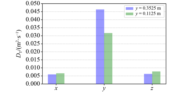
 Fig.1 The domain with (a) imposed initial and (b) boundary conditions for methods 2 and 1, respectively.Fig.2 A visual comparison of instantaneous volume fraction fields in the different beds studied. (a) The HiVoid case with smaller sand corresponds to the solids used in the experiments of Sette et al. [33], and (b, c) the LoVoid cases with larger sand corresponds to the solids used in the experiments of Martinez Castilla et al. [37]. The LoVoid-small-nozzle case (c) employs “nozzle” inlet boundary condition instead of the uniform “porous plate” inlet boundary condition used in the other cases (a, b).Fig.3 Experimental [33] and simulated (current work) values of the solids lateral dispersion coefficient for the HiVoid cases, extracted using methods 2 (DispTrans) and 3 (CondSteady).Fig.4 Experimental [37] and simulated (current work) values for the denser bed (LoVoid cases). The experimental error bars indicate lower and upper bounds for the method used (more information is provided in the ESM).Fig.5 A collected comparison of the different analysis methods tried for all the available data sets. The solid black lines indicate the experimentally obtained DL for the HiVoid case and the experimentally obtained uncertainty interval for DL for the LoVoid cases (Fig. 4).Fig.6 The computed turbulent dispersion DT in each direction (averages along two planes at different heights in the bed).
/
| 〈 |
|
〉 |